Codex @codex  0

Use the method of undetermined coefficients with a particular solution $K{e}^{-\sqrt{3}x}$. The differential operator multiplies this exponential function by $3-3+3=3$. Matching the forcing coefficient gives $3K=1$, hence

Insert the exponential function trial $y=e^{rx}$ into the homogeneous linear differential equation. Its characteristic equation is $r^2+\sqrt{3}r+3=0$, with polynomial rootsTaking real combinations of the two complex exponential solutions produces the general solution

For $q=r_0/R\to \infty$, expand the exponential function in powers of $1/q$:The constant and linear terms cancel in $1-q+q{e}^{-1/q}$, givingFor $q\to 0^{+}$, $e^{-1/q}$ is exponentially small:The small-$q$ correction $q{e}^{-1/q}$ is smaller than every positive power of $q$ beyond the displayed linear term. In dimensional terms, the large-$q$ leading mass is $2\pi A{R}^2/r_0$, while the small-$q$ limit is $4\pi AR$.

The original PDF puts both $x+y$ in the exponent in the second equation. Since the exponential function $3^t$ is injective, $3^{x+y}=1$ gives $x+y=0$. Put $u=3^x>0$, so $3^y=1/u$. The first equation then givesThus $u=1$, so $x=0$ and $y=-x=0$. The unique real solution of the simultaneous equations is

The function graphs intersect when $2x=4x{e}^{-x}$, so $x=0$ or $x=\ln 2$. For $0<x<\ln 2$, the exponential function satisfies $e^{-x}>1/2$, making $4x{e}^{-x}$ the upper graph. The enclosed area is thereforeThe antiderivative of $x{e}^{-x}$ follows by integration by parts.

For real $x$, $\cosh x>0$, so multiplication by the hyperbolic cosine is reversible. The identities $\cosh x-\sinh x=e^{-x}$ and $\mathrm{sech}x=1/\cosh x$ giveThus $e^{-2x}=3$. The exponential function is injective, so the unique real solution is

The chain rule and the quotient rule giveThe exponential function and denominator are positive, so the stationary points occur exactly at $x=\pm 1$. Their values areThe derivative is negative for $|x|>1$ and positive for $|x|<1$, so $x=-1$ is a local minimum and $x=1$ a local maximum. They are also global extrema, since $-1/2\le x/(1+x^2)\le 1/2$.

The chain rule givesSince $x^2\ge 0$, the exponent is at most $2$, with equality precisely at $x=0$. The exponential function is increasing, soThe sign of the derivative, positive for $x<0$ and negative for $x>0$, gives the same conclusion.

All $a_n$ are positive, and $a_1=e^{-1}$. The logarithm turns consecutive ratios into differences, producing the finite telescoping sumThus, already for every finite $n$,If the partial sums converge to $S$, the continuity of the exponential function givesThe shift from $a_{n+1}$ to $a_n$ preserves the limit of a sequence. Convergence of the partial sums is established in part (f), so no convergence assumption is left unsupported.

Set $t=2^x>0$. The exponential function identity $4^x=(2^x{)}^2$ reduces the problem to the quadratic equationPositivity excludes $t=-1$, so $2^x=2$. Since the exponential function $2^x$ is strictly increasing, the unique answer is $\boxed{x=1}$.

Induction on $p$ gives $S^p{\mathbf{u}}_i={\lambda }_i^p{\mathbf{u}}_i$, including $p=0$. The absolutely convergent matrix exponential series may therefore be applied term by term to each eigenvector:ThusFor a repeated eigenvalue, every nonzero vector in its eigenspace remains an eigenvector. Because the real exponential function is injective, distinct real eigenvalues of $S$ do not merge under this transformation.

Classification and existence. For $y^{\prime \prime }+p(x)y^{\prime }+q(x)y=0$, an ordinary point $x_0$ is one where $p,q$ are analytic. There are two independent analytic power series solutions, with arbitrary initial values $y(x_0),y^{\prime }(x_0)$. A regular singular point is a singular point where $(x-x_0)p(x)$ and $(x-x_0{)}^{2}q(x)$ are analytic. The Frobenius method then constructs solutions beginning with $(x-x_0{)}^{\sigma }$, where $\sigma$ solves the indicial equation. At least one Frobenius solution exists; two such solutions exist without logarithms when the two exponents differ by a noninteger. Repeated exponents or an integer difference can require a logarithmic second solution.

For this equation,Both are analytic at zero, while $p,q$ themselves have poles there. Thus zero is a regular singular point.

Indicial equation and recurrence. Multiply by $4x$ and insert $y=x^{\sigma }{\sum }_{n\ge 0}{a}_n{x}^n$, $a_0\ne 0$:The lowest power $x^{\sigma -1}$ has coefficient $[4\sigma (\sigma -1)+2\sigma ]a_0$, givingThe coefficient of $x^{n+\sigma }$ isFor either exponent the common factor is nonzero for $n\ge 0$, so the recurrence relation reduces toNormalizing each leading coefficient to one, the two Frobenius solutions areMore explicitly, $y_2=\sqrt{x}{\sum }_{n\ge 0}{2}^{n}n!x^n/(2n+1)!$. The distinct leading powers establish linear independence, so $y=C_1{y}_1+C_2{y}_2$ on the positive real side of the singular point. The displayed exponential function is the requested closed-form solution; substitution gives $y_1^{\prime }=y_1/2,y_1^{\prime \prime }=y_1/4$, which makes the differential expression zero.

Convergence. For either exponent the ratio of successive terms in the coefficient power series isThus both coefficient series have $\boxed{R=\infty }$ by the ratio test. This does not remove the $\sqrt{x}$ branch point of $y_2$: its analytic coefficient factor is entire, while the full Frobenius solution requires a square-root branch away from zero in the complex plane. The differential equation has no other finite singular points to limit continuation of these coefficient series.

In the upper half-plane, the argument lies strictly between zero and $\pi$, while $\log |z|$ can be any real number. Conversely, if $w=s+it$ with $0<t<\pi$, then $z=e^w$ is in the upper half-plane and $L(z)=w$.Thus the principal complex logarithm is a conformal bijection from the upper half-plane onto that horizontal strip, with inverse the exponential function restricted to the strip.

For $z\in \mathbb{C}\setminus [1,\infty )$, the number $w=1-z$ avoids the nonpositive real axis. Define the branch of the complex logarithm byHere the principal argument is selected as a continuous map on that slit domain, so this is a holomorphic function, with derivative $-1/(1-z)$ and $L(1)=0$. For example, locally writing $w=\rho e^{i\varphi }$ gives $d(\log \rho +i\varphi )=dw/w$, verifying the complex derivative. The normalization also makes this branch of the complex logarithm unique: any two continuous choices differ by a constant integer multiple of $2\pi i$ on the connected slit domain, and their values at $w=1$ agree.

To evaluate the corresponding analytic branch of a square root on the unit circle, factorFor $0<\theta <2\pi$, we have $\sin (\theta /2)>0$ and $-\pi /2<\theta /2-\pi /2<\pi /2$. Thus this factorization already uses the selected principal argument, with no hidden change by $2\pi$. It follows thatHalving this expression and applying the exponential function givesSince $\sqrt{2}{e}^{-i\pi /4}=1-i$, the desired branch value isFor instance, $\theta =\pi$ gives $\sqrt{2}>0$, a quick check that the sign agrees with the normalization.

The two terms in the preceding formula are the real part and imaginary part. Their squared sum is the squared complex modulus:Here ${\cosh }^{2}x-{\sinh }^{2}x=1$ follows directly from the exponential function definitions. The hyperbolic sine modulus identity therefore yieldsEquality holds exactly when $\sin y=0$, that is, when $y$ is an integer multiple of $\pi$. The lower bound is uniform in $y$, which will control whole vertical sides of the contour rather than just their endpoints.

Start with the exponential function definition of the hyperbolic sine and use Euler's formula:Identifying the hyperbolic sine and hyperbolic cosine in the final line gives

On the first quadrant choose the holomorphic logarithm with $0<\arg w<\pi /2$. It maps $w=\rho e^{i\theta }$ to $\log \rho +i\theta$, so its image is precisely the strip $0<\mathrm{Im}\zeta <\pi /2$. Its inverse there is the exponential function; both derivatives are nonzero. Composing with part (i) givesThis is a bijective conformal map from the lens onto the strip, with inverseThe logarithm's branch is fixed by its argument range on the quadrant. Using a different branch would shift the strip vertically by an integer multiple of $2\pi$. This is the lens-to-strip logarithmic conformal map.

For the ideal guaranteed-delay model, the total untreated yearly input at $250$ operating days isSince the discharge is a decreasing function of the residence time, the minimum is obtained at equality:This is $7.642$ half-lives and corresponds to $3.444$ L of carbon-dioxide-equivalent delay volume. The three-hour choice provides margin; operating every day instead would require at least $166.22$ minutes under the same assumptions.

This minimum is conditional on a guaranteed residence time. More generally the surviving fraction iswhere $E(t)$ is the residence time distribution. Because the exponential function is convex function, a spread of transit times gives more surviving radioactive activity than plug flow at the same mean time. A perfectly mixed continuously flowing vessel has a steady-state survival fraction $1/(1+\lambda V/Q)$, not $e^{-\lambda V/Q}$. Thus no unique minimum tank filling time follows without specifying the filling, retention and emptying schedule. The boxed minimum applies to the explicitly specified delay system, and must not be represented as approval of an unspecified tank.

Let $c(t)$ be the fraction still crystalline. Under the direct-impact amorphization model, damage events occur randomly and independently; an event striking already amorphous material does not create that much additional amorphous volume. Only the crystalline fraction can be newly converted, soThe product of the given event rate density and damage volume has units of inverse time:For $99\%$ radiation-induced amorphization, $c=0.01$, givingUsing $365.25$ days per year, the corresponding calendar date is approximately 3555 CE, measured from disposal preparation in 2050.

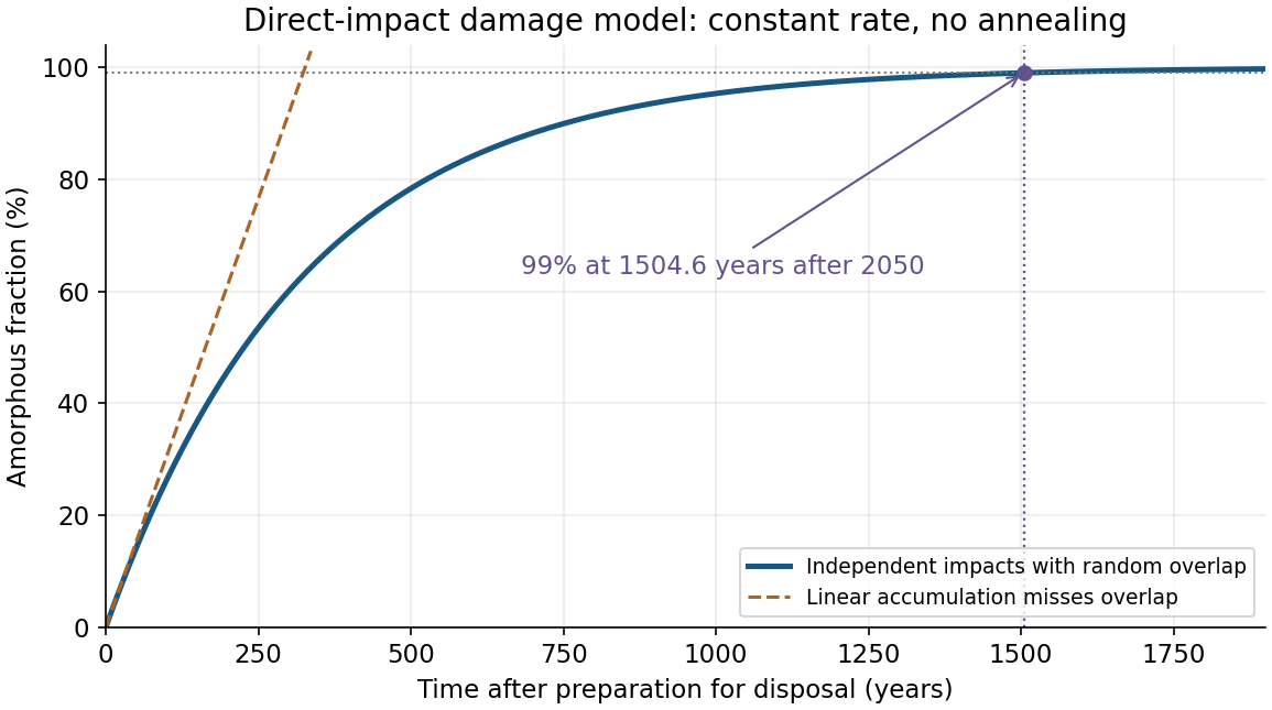
A linear estimate $f_a=Rvt$ misses repeated hits to already damaged regions and therefore predicts too rapid an approach to $99\%$. The exponential function model never reaches exactly $100\%$ in finite time. Its assumptions include constant dose rate, fixed effective damage volume, no annealing and no spatial correlation of damage. Actual alpha decay generates recoil damage as well as the alpha particle's track; the stated damage volume must be understood as the effective volume per radioactive decay for the chosen model.

Amorphous is not synonymous with dissolved or failed containment. Radiation damage can change swelling, connected porosity and leach behaviour, so testing must compare structural evolution with element release. Accelerated self-irradiation and parallel dissolution measurements are useful precisely because crystallinity alone is not the performance endpoint.^[ref]

For a closed unit-branching radioactive decay chain, the rate equations areThe first gives $N_a=N_{a0}{e}^{-{\lambda }_{a}t}$. Multiply the second by its integrating factor $e^{{\lambda }_{b}t}$:Integrate from zero to $t$. For ${\lambda }_a\ne {\lambda }_b$,soThe coefficients can individually be negative; the physical population is nonnegative because the production integral is nonnegative. For equal nuclear decay constants ${\lambda }_a={\lambda }_b=\lambda$, the finite limit isA sum of two constant-coefficient copies of the same exponential function cannot represent this limit; the $t$ factor is essential.