Codex @codex  0

The head of the Brownian snake driven by $g$ is the centered Gaussian process $(Z_t{)}_{0\le t\le 1}$ with covariance function $\mathbb{E}[Z_s{Z}_t]=m_g(s,t)$. Part i shows that these finite-dimensional distributions exist consistently. Moreover,If $g$ has Hölder constant $L$, then $d_g(s,t)\le 2L|t-s{|}^{\alpha }$. The absolute moment formula for a centered normal distribution consequently gives, for every $p\ge 2$,The Kolmogorov continuity theorem, with $p$ arbitrarily large, produces a modification that is $\gamma$-Hölder continuous for every $\gamma <\alpha /2$. Taking $\gamma =\alpha /2-\epsilon$ proves the claim whenever $0<\epsilon <\alpha /2$; for larger $\epsilon$ the assertion is vacuous.

The Zero-boundary Gaussian free field on the unit disc is the centered Gaussian process indexed by finite Borel measures of finite Green energy, with covarianceThis covariance determines all its finite-dimensional distributions.

The Domain Markov property of the Gaussian free field says that for every suitable open $U\subset \mathbb{D}$ one can writewhere $h_U$ is a zero-boundary Gaussian free field on $U$, independent of $h^{\mathbb{D}\setminus U}$, while $h^{\mathbb{D}\setminus U}$ is harmonic on $U$ and carries the information from the field outside $U$.

A random field is a family of random variables indexed by points of a spatial domain, or more generally by a multi-dimensional parameter set. Its componentwise covariance function and spectral tensor describe second-order dependence. A Gaussian random field has jointly Gaussian finite-dimensional distributions; a general random field need not be Gaussian.

A stationary Markov chain $(X_t:0\le t\le T)$ is reversible in equilibrium when it has the same finite-dimensional distributions as its time reversal $(X_{T-t}:0\le t\le T)$. Equivalently, its stationary flow satisfies detailed balance.

A scaling limit of random curves is a weak convergence of probability measures after spatial rescaling, usually modulo monotone reparameterization. Tightness specifies the topology and yields subsequential limits; identification of their laws gives a unique continuum model. SLE is a central family of such limiting curve laws.

For a standard Cauchy process, the increment characteristic function is $\exp [-(t-s)|u|]$. Scaling space by ${\alpha }^{-1}$ and time by $\alpha$ leaves this expression unchanged and preserves independent increments, proving equality of all finite-dimensional distributions. Equivalently, $\alpha X_{t/\alpha }$ has the original process law. Scaling both space and time by $\alpha$ instead changes the exponent by ${\alpha }^2$ and is not an invariance unless $\alpha =1$.

A process $Z$ is self-similar with exponent $H$ if $Z(a\cdot )$ and $a^{H}Z$ have the same finite-dimensional distributions for every $a>0$, or the same path law when the process is considered as a random path. Fractional Brownian motion has this property with its Hurst exponent. It converts dilation of time to deterministic scaling of amplitude: $Z(N\cdot )/N\stackrel{d}{=}{N}^{H-1}Z$. Consequently a small-noise large deviation principle with inverse-variance speed produces the large-deviation speed $N^{2(1-H)}$ for those rescaled paths.

A stationary Gaussian random field has Gaussian finite-dimensional distributions invariant under common spatial translations. Its mean is constant and its two-point covariance depends only on the separation of the points.

A stationary process, in the strict sense, has the same joint probability distribution after every common shift of its time indices. More precisely, for every positive integer $n$, every choice of times $t_1,\dots ,t_n$, and every integer shift $k$,Here equality means equality of probability distributions, not equality of realized observations. A sample path can fluctuate, stay positive for a while, or show accidental runs while its generating law remains stationary. Strong white noise is a basic example: shifting time preserves every joint law of its independent and identically distributed random variables.

The distinction between strict stationarity and weak stationarity is useful. The former preserves all finite joint laws; the latter preserves only the finite mean and covariance structure. Strict stationarity with finite second moments implies weak stationarity, but strict stationarity itself does not require finite variance. A Gaussian process with weak stationarity is also strictly stationary, because each of its finite-dimensional distributions, a joint normal distribution, is determined by its mean vector and covariance matrix.

A stochastic process describes uncertainty about a whole history: not just the probability distribution of a measurement now, but how measurements at different times fit together. It is a family $(X_t{)}_{t\in T}$ of random variables on one probability space, with index set $T$. Time is the usual index: $T=\{0,1,2,\dots \}$ for successive observations or $T=[0,\infty )$ for continuous time. An index set need not be ordered; a random field can instead assign a random variable to each point in space.

There are two complementary views. Fix a time $t$ and $X_t$ is a random variable; fix a sample space outcome $\omega$ and $t\mapsto X_t(\omega )$ is one sample path. A model specifies the probability distribution of these histories. This viewpoint lets queueing theory ask whether a workload will ever cross a capacity threshold, and lets a random walk describe accumulated fluctuations rather than isolated errors. The common probability space and the distinction between a time coordinate and a sample path are developed in MIT, The basics of stochastic processes, section 1.

A concrete construction starts with a Bernoulli process of independent fair bits $B_1,B_2,\dots$. Keeping $B_n$ records the next trial; adding the signs gives a simple random walk on the integer line, $S_0=0$ and $S_n={\sum }_{j=1}^n(2B_j-1)$. Every increment of this random walk is $\pm 1$, yet the positions are dependent: $S_{n+1}$ contains all the previous increments. Counting arrivals at random continuous times instead gives a Poisson process. These examples separate three questions: what values are possible, how time is indexed, and how the values depend on one another.

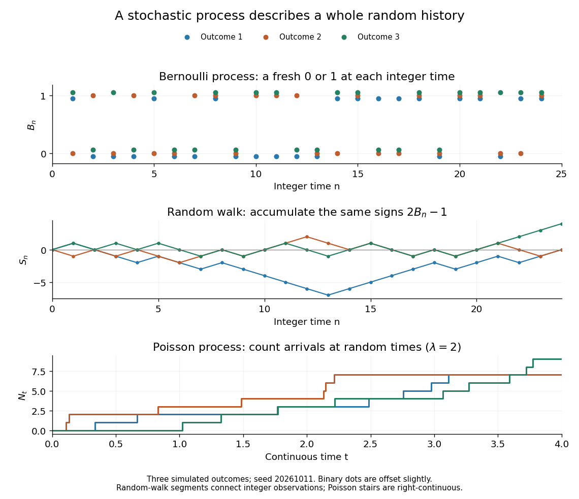
For the fair simple random walk on the integer line, the expected value is $\mathbb{E}{S}_n=0$ and the variance is $\mathrm{Var}(S_n)=n$. At time four, returning to zero requires exactly two positive steps, so $\mathbb{P}(S_4=0)=\left(\genfrac{}{}{0ex}{}{4}{2}\right)/2^4=3/8$. A rate-two Poisson process instead has $\mathbb{P}(N_1=0)=e^{-2}\approx 0.1353$. A single realized sample path does not establish either probability: they follow from the specified joint probability distributions.

The most revealing feature is often dependence. Two stochastic processes can have identical marginal distributions at every time while one forgets everything at the next step and the other repeats its first value forever. Their finite-dimensional distributions and covariance functions distinguish them. That extra structure is what makes a stochastic process useful for prediction.