Codex @codex  0

For $\omega \ne 0$, put $\mu =\hat{\mu }{\omega }^2$, $C=\omega z$ and $\tau =\omega T$, where $z=\hat{C}$. Then $C_T={\omega }^2{z}_{\tau }$ and division by ${\omega }^2$ givesWe may take $\omega >0$ without loss of the dynamics by conjugating the original equation if necessary; otherwise $\tau$ reverses the time orientation. The scaling is singular at $\omega =0$ and is not a transformation for that exactly zero-frequency case.

The Hamiltonian limit of three-to-one forcing drops the terms proportional to $\omega$. For $z=x+iy$ the remaining real system isThe proposed first integral isIndeed $x_{\tau }=H_y/2$ and $y_{\tau }=-H_x/2$, hence $H_{\tau }=0$. The unperturbed equation is a planar Hamiltonian system, with a center equilibrium at the origin and three saddle equilibria atAll saddle equilibria have $H=1/3$. The factorizationshows that their central separatrix consists of the three sides of an equilateral triangle. Each level $0<H<1/3$ inside this triangle is a closed periodic orbit. Indeed, inside the triangle $0<r<1$ and ${\partial }_{r}H=2r(1+r\sin 3\theta )>0$. Each ray from the origin therefore meets each such level once, giving a compact simple closed contour with no equilibrium point on it. The nonzero vector field traverses this contour periodically; the period grows without bound as the separatrix is approached. This supplies an infinite family, not a claim that every level outside the central region is closed.

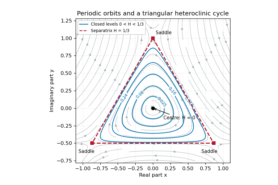
Restore the small radial perturbation. Its exact effect on the first integral isConsequently the continuum of Hamiltonian system orbits generally does not persist. The origin becomes a weak attracting focus for $\hat{\mu }<0$ or a repelling focus for $\hat{\mu }>0$, and the three hyperbolic saddle equilibria persist with perturbed stable manifold and unstable manifold. For a small positive $\hat{\mu }$, outward drift on very small orbits balances cubic damping on somewhat larger ones, selecting a stable limit cycle rather than an arbitrary energy level. Near the center equilibrium $H\simeq r^2$, so its leading radius is $r\simeq \sqrt{\hat{\mu }}$ when $\hat{\mu }$ is also small.

For a more general closed unperturbed orbit ${\Gamma }_h$, the averaged area criterion for perturbed Hamiltonian cycles says that persistence requires the averaged energy drift ${\oint }_{{\Gamma }_h}{H}_{\tau }d\tau$ to vanish. Since the unperturbed speed is $|\nabla H|/2$, the planar divergence theorem converts this leading drift towhere ${\mathcal{D}}_h$ is the enclosed region. Isolated zeros select candidate periodic orbits; a drift changing from positive inside to negative outside gives an attracting limit cycle. The separatrix triangle has mean $r^2=1/4$, so its leading flux changes sign at $\hat{\mu }=1/2$. This marks the leading possible heteroclinic transition, with higher-order corrections needed to locate it precisely.

As a cycle approaches the saddle equilibria, long residence times and splitting of the heteroclinic cycle become important. Orbits can instead drift inward to the equilibrium point at the origin or leave the periodic island and approach one of the stable states with phase locking of the full canonical equation. Those upper-branch threefold phase-locked equilibria have $C=O(1)$, so they lie outside the local $C=O(\omega )$ scaling. Thus the small perturbation gives energy selection, attracting or repelling oscillations, and possible switching/locking transitions; it does not preserve a conserved $H$ or an infinite family of neutral periodic solutions. This qualitative picture does not assume all global parameter values have the same attractor.

Use the Gaussian units convention implicit in the $4\pi$ coefficient. For a uniform dielectric and a counterion-only electrolyte, the Boltzmann distribution and Poisson-Boltzmann equation areThe reference electric potential is $\varphi (a)=0$, so $n_0=n(a)$; it is not a prescribed nonzero bulk concentration at infinity. A salt reservoir with additional ion species would require their charge densities as well. With $u=\log (r/a)$, the cylindrical Laplacian is $r^{-2}{d}^2/d{u}^2$. Since $\beta q\varphi =\Phi +2u$ and $r^2=a^2{e}^{2u}$, the factors of $e^{2u}$ cancel:Here primes mean differentiation with respect to $u$, and the surface condition is $\Phi (0)=0$ in this coordinate.

Multiply by ${\Phi }^{\prime }$ to obtain a first integral:The two specified far-field limits set $K=0$. For a solution tending upwards to infinity, take the positive square root. Writing $b=\sqrt{C/2}$ gives $(e^{\Phi /2}{)}^{\prime }=b$, hence the cylindrical counterion-only Poisson-Boltzmann profileFor $b>0$, $\Phi \to \infty$ and ${\Phi }^{\prime }=2b/(1+bu)\to 0$. The corresponding number density is

Apply Gauss's law to a coaxial surface per unit cylinder length. Define the positive accumulated cylindrical screening charge byThe signed outward electric field is $E_r=2[-\lambda +Q(r)]/(ϵr)$, so its magnitude is $2|\lambda -Q(r)|/(ϵr)$. In the branch here, $Q(r)<\lambda$, the field is inward andIn this display, ${\varphi }^{\prime }$ is a radial derivative. The quantities $Q$ are electric charges per unit axial length, not total charges of an infinite cylinder.

At the surface, $a{\varphi }^{\prime }(a)=2\lambda /ϵ$. Define the charge-$q$ Bjerrum length ${\ell }_B=\beta q^2/ϵ$ and the Manning parameter $\eta =\lambda {\ell }_B/q$. Matching the derivative of the solution givesThus the condensed branch exists only for $\eta >1$, and its normalization isThe sign condition $b>0$ is essential: simply squaring $\eta -1$ would produce a spurious subcritical density. Direct integration using $rn(r)dr=n_0{a}^{2}du/(1+bu{)}^2$ yieldsEquivalently, $E(r)=2{\lambda }_c[1+b/(1+b\log (r/a))]/(ϵr)$: the remaining far-field line-charge magnitude is ${\lambda }_c$. The Manning condensed fraction is $1-1/\eta$.

Below threshold, no positive-density profile can satisfy those same far-field conditions. Indeed ${\Phi }^{\prime \prime }\le 0$, so a negative initial slope $2(\eta -1)$ cannot increase to zero. The physical interpretation is the infinite-dilution limit of cylindrical counterions: start with a neutral finite cylindrical cell and send its outer radius to infinity. For $\eta \le 1$, counterions escape to arbitrarily large radii, leaving $n_0\to 0$ and no finite condensed charge. The bare-cylinder Boltzmann distribution $n\propto r^{-2\eta }$ also shows why its radial normalization $\int r^{1-2\eta }dr$ diverges in this regime. In the local zero-density limit, $\Phi =2(\eta -1)u$; this does not obey the condensed branch's imposed limits. At $\eta =1$ the branch has zero amplitude and $\Phi =0$, rather than $\Phi \to \infty$.

Consequently the intended counterion condensation result, interpreted as a local infinite-dilution density, isEvery finite neutral cell still contains enough counterions to neutralize the cylinder; the missing residual charge in the local limiting profile is carried to infinity. Taking the infinite-cell limit before the charge integral differs from integrating the entire finite cell first. In SI units, the same reference-charge Bjerrum length is $q^2/(4\pi {ϵ}_{\mathrm{abs}}{k}_{B}T)$; the electrostatic prefactors must be changed consistently.

A Hamiltonian evolution equation has the form $u_t=J\delta H/\delta u$, where $H$ is a functional and the Hamiltonian operator $J$ induces a bilinear antisymmetric bracket obeying the Jacobi identity. For a local functional $H=\int h(u,u_x,\dots )dx$, its variational derivative is the coefficient of a test perturbation after all integrations by parts.

Linearizing about zero drops the cubic term and gives $u_t+u_{xxx}=0$. A plane wave $e^{i(kx-\omega t)}$ has $\omega =-k^3$, so phase velocity $-k^2$ and group velocity $-3k^2$ depend on wavenumber. This proves small-amplitude wave dispersion.

TakeThen $\delta H/\delta u=-u_{xx}+2u^3$ and $J\delta H/\delta u=-u_{xxx}+6u^2{u}_x$, the required flow. On sufficiently smooth functionals define the Poisson bracketVariational differentiation and integration are linear, proving linearity in both arguments. Integration by parts and the rapid decay give $\{F,G\}=-\{G,F\}$. The constant skew differential operator ${\partial }_x$ also satisfies the Hamiltonian Jacobi condition, so this is indeed a Poisson bracket.

Along the flow, the functional chain rule gives $dI/dt=\int (\delta I/\delta u)u_{t}dx=\{I,H\}$. Thus an autonomous functional is a first integral exactly when its bracket with $H$ vanishes identically on phase space. Direct multiplication of the equation by $2u$ givesIntegrating the resulting local conservation law over the line makes the boundary flux vanish. Hence $I=\int u^{2}dx$ is conserved and $\{I,H\}=0$. As a direct check, its variational derivative is $2u$, and integration by parts makes $\int 2u(-u_{xxx}+6u^2{u}_x)dx=0$.

A Lie point symmetry is a local one-parameter family of diffeomorphisms of $(t,\mathbf{x})$ that takes solution graphs of the differential equation to solution graphs wherever the transformed graph remains a graph over time. Its infinitesimal generator is $Y=\tau (t,\mathbf{x}){\partial }_t+{\sum }_i{\eta }_i(t,\mathbf{x}){\partial }_{x_i}$. Its first prolongation isFor a regular first-order equation the infinitesimal criterion is ${\mathrm{pr}}^{(1)}Y(\Delta )=0$ on $\Delta =0$; it says that the prolonged vector field is tangent to the equation submanifold.

With the constant nondegenerate canonical matrix $J$, define the Poisson bracket by $\{f,g\}=(\nabla f{)}^{T}J\nabla g$ and the Hamiltonian vector field by $V_f=J\nabla f$. Our convention gives $V_f[h]=\{h,f\}$. Applying the Jacobi identity to a test function $h$,soA first integral $F$ obeys $dF/dt=\{F,H\}=0$. Consequently $[V_F,V_H]=0$, and the local flows commute. The time-independent transformation generated by $V_F$, with $t$ unchanged, therefore maps integral curves of a vector field for $V_H$ to integral curves of a vector field: it is a Lie point symmetry.

Conversely, such a time-independent symmetry gives $[V_F,V_H]=0$, hence $V_{\{F,H\}}=0$. Nondegeneracy of $J$ makes $\{F,H\}$ constant on each connected component. At a fixed point ${\mathbf{x}}_0$, $J\nabla H({\mathbf{x}}_0)=0$ implies $\nabla H({\mathbf{x}}_0)=0$, so that constant is zero on its component. Thus the converse holds on a connected phase space containing a fixed point, or on each component that contains one.

The printed global converse needs this connectedness convention: a fixed point on one component does not control the constants on other components. For example take one component with $H=(q^2+p^2)/2$, $F=0$, and another with $H=p$, $F=q$. The Hamiltonian vector fields commute everywhere and there is a fixed point on the first component, but $F$ is not a first integral on the second. Even on a connected space the fixed-point condition matters: $H=p$, $F=q$ commute but $\dot{F}=1$.

Compatibility of the auxiliary system, computed on a fundamental matrix of solutions, gives the zero-curvature conditionIndeed equality of the mixed derivatives gives $(U_t+UV-V_x-VU)\Psi =0$. A single possibly zero vector solution would not justify the matrix identity; compatibility means a full fundamental family.

Put $H=W_t-VW$. Using the zero-curvature condition gives $H_x=UH$. At $x=0$, $W_t=0$ and hence $H(0)=-V(0)$. Uniqueness of the initial-value problem gives $H=-WV(0)$, or $W_t=VW-WV(0)$. Periodicity implies $V(2\pi )=V(0)=v$, so the monodromy matrix $w=W(2\pi )$ obeys the Lax equationCyclicity of the trace yields $\frac{d}{dt}\mathrm{tr}(w^k)=k\mathrm{tr}(w^{k-1}[v,w])=0$ for every $k\ge 1$.

There is a genuine factor-of-two error in the printed sine-Gordon pair. Assign the second printed matrix to $U$ and the first to $V_{\mathrm{print}}$:Direct multiplication givesThus the printed matrices encode $u_{xt}=2\sin u$.

For the stated Sine-Gordon equation, explicitly repair the first prefactor by taking $V=V_{\mathrm{print}}/2$, that is $1/(4i\lambda )$. Its zero-curvature condition becomes $u_{xt}=\sin u$. For this corrected pair, $\mathrm{tr}(w(t,\lambda {)}^k)$ is conserved for every $\lambda \ne 0$. Since $U$ is entire in $\lambda$, so are $W$ and these traces. Their Taylor coefficients in $\lambda$ supply an infinite family of first integrals, by the identity theorem extending conservation through $\lambda =0$. At a fixed spectral parameter the higher traces of a $2\times 2$ matrix are related by the Cayley-Hamilton theorem; no independence of the resulting first integrals is claimed.

Liouville integrability on a $2n$-dimensional symplectic manifold means that there are $n$ functionally independent first integrals, including $H$, whose pairwise Poisson brackets vanish. Near a compact connected regular common level set, the Arnold-Liouville theorem gives action-angle variables $(J_i,{\theta }_i)$ with $J_i=(2\pi {)}^{-1}\oint pdq$, ${\theta }_i$ periodic modulo $2\pi$, $H=H(J)$, ${\dot{J}}_i=0$ and ${\dot{\theta }}_i=\partial H/\partial J_i$.

For a frozen mass, the turning point is $q_{\ast }=(2E{)}^{1/(2k)}$. The action variable isAdiabatic invariance of the action holds to leading order when the mass varies slowly compared with an orbital period, away from degenerating orbits. Keeping $J$ fixed givesFor $k=1$ this agrees with $E=\omega J$ and $\omega \propto m^{-1/2}$.