Codex @codex  0

Put $s=\sqrt{b}$. The two fixed points on the invariant line $x=0$ are $P_{+}=(0,s)$ and $P_{-}=(0,-s)$. There are also $Q_{\pm }=(\pm \sqrt{b-a^2/4},-a/2)$ when $a^2<4b$. At equality they coalesce with $P_{-}$.

The Jacobian matrix isAt $P_{+}$ its eigenvalues are $-a-2s$ and $2s$, so it is always a saddle equilibrium. At $P_{-}$ they are $2s-a$ and $-2s$, so it is a saddle equilibrium for $a<2s$ and a stable node for $a>2s$, with a zero eigenvalue at $a=2s$.

At $Q_{\pm }$ the characteristic equation is ${\lambda }^2+a\lambda +4b-a^2=0$, givingFor $0<a^2<16b/5$ these points are stable spirals; for $16b/5<a^2<4b$ they are stable nodes. At $a^2=16b/5$ the double negative eigenvalue has only one independent eigenvector, so these are improper stable nodes. When $a=0$ they are center equilibria, as established in part (iii). Thus the collision at $\boxed{a^2=4b>0}$ changes both the number and stability of fixed points; it is the bifurcation classified below.

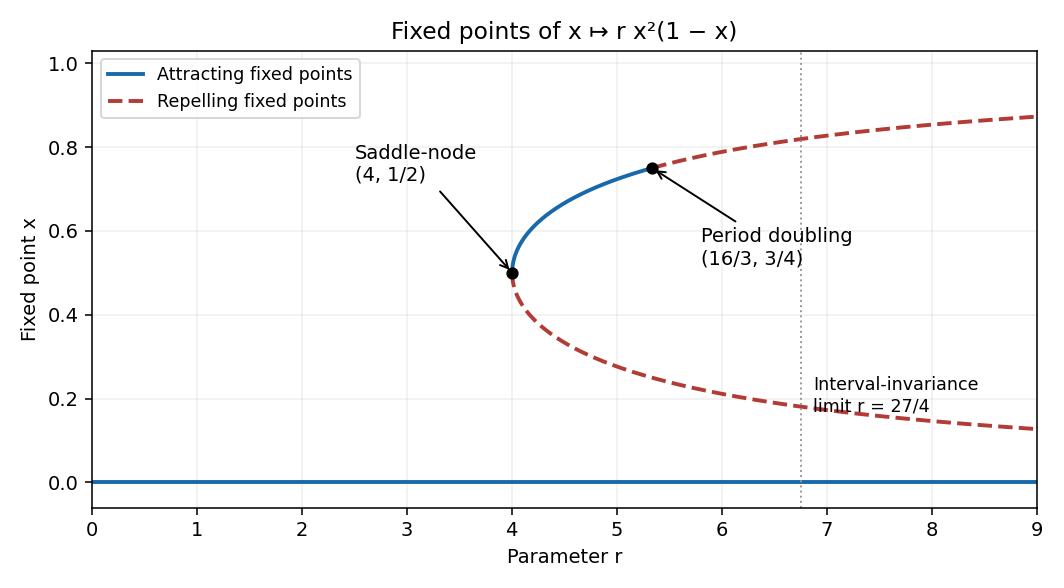
The fixed points satisfy $x[rx(1-x)-1]=0$. There is always $x=0$, and the other branches areThey coincide at $(r,x)=(4,1/2)$. For $0<x<1$, $F(x)>0$ and its maximum occurs at $x=2/3$, with value $4r/27$. Consequently $\boxed{F((0,1))\subset (0,1)⟺0<r<27/4}$; equality at the upper endpoint fails because the maximum is attained inside the interval.

The fixed-point multiplier at zero is zero, so zero is attracting for every $r>0$. On either nonzero branch,The lower branch has multiplier greater than one for $r>4$ and is repelling. The upper branch is attracting for $4<r<16/3$, reaches multiplier $-1$ at $x=3/4$, and is repelling for $r>16/3$. At $r=4$ the multiplier is $+1$, and the two branches are created in a saddle-node bifurcation. The fixed point there is attracting from one side and repelling from the other: $F(x)-x=-4x(x-1/2{)}^2$.

The second change is a supercritical period-doubling bifurcation at $\boxed{(r,x)=(16/3,3/4)}$. To check its type, expand at that fixed point. The local map has quadratic coefficient $a=-20/3$ and cubic coefficient $b=-16/3$ when the multiplier is $-1$. Its second iterate has cubic coefficient $-2(a^2+b)=-704/9<0$. The multiplier decreases through $-1$ as $r$ increases, so a small attracting two-cycle is born on the $r>16/3$ side. These exhaust the fixed-point bifurcations, since their multipliers have no other crossings of $\pm 1$.

An interval covering relation $I\to J$ means $F(I)\supseteq J$. The associated directed graph has one vertex for each interval and an edge $i\to j$ for each covering. Its transition matrix is $A_{ij}=1$ when that edge exists, and zero otherwise. Matrix multiplication counts walks; thus $\boxed{\mathrm{tr}(A^n)}$ counts closed length-$n$ itineraries, with a distinguished starting vertex.

To see how itineraries force periodic orbits, a continuous map covering a closed interval has a closed subinterval mapping onto it: choose successive first/last crossings of its endpoints. Pull these subintervals back along a closed walk. This yields $K\subseteq I_{i_0}$ with $F^n(K)\supseteq I_{i_0}\supseteq K$. At the two preimages of the ends of $K$, $F^n(x)-x$ has opposite weak signs; the intermediate value theorem gives a fixed point of $F^n$.

A graph alone does not give an exact count of periodic points for a general continuous map: extra oscillations or a fixed interval can create additional points. For example on $I=[0,1]$, both $F(x)=x$ and $F(x)=1-x$ have matrix $A=(1)$; the first has infinitely many fixed points and the second only one. Distinct itineraries give distinct points when their interval interiors are disjoint and the periodic orbit avoids shared endpoints. In that setting, $\mathrm{tr}(A^n)$ is a guaranteed lower bound, not a universal equality. Likewise, the primitive-word count $(1/n){\sum }_{d\mid n}\mu (d)\mathrm{tr}(A^{n/d})$ counts guaranteed least-period itineraries under this separation condition. With overlapping intervals, even distinctness needs qualification. This is the scope of counting cycles in an interval covering graph.

For the first five-cycle, put $I_j=[x_j,x_{j+1}]$, $0\le j\le 3$. The graph and matrix areThe four traces are $1,3,7,15$. Shared endpoints have least period five, so they do not spoil the distinctness argument for the requested periods. Primitive cyclic itineraries are: $3$ for period one; $(3,2)$ for period two; $(3,1,2)$ and $(3,3,2)$ for period three; $(0,1,2,3)$, $(3,3,1,2)$ and $(3,3,3,2)$ for period four. Consequently the monotone five-cycle interval covering pattern guaranteesThese words specify the successive intervals containing their points; cyclic rotations denote the same orbit.

There is a horseshoe for an interval map for $F^2$: both $I_2$ and $I_3$ cover $I_2\cup I_3$ under that iterate, and their interiors are disjoint. Repeated binary choices produce at least $2^n$ separated length-$n$ itineraries for the second iterate, hence positive topological entropy, at least $(\log 2)/2$ for $F$. Thus the dynamics are chaotic in this standard interval-map sense. No conclusion of global transitivity on all of $\mathbb{R}$ follows.

A one-step horseshoe is not guaranteed if that is the intended definition. For example the unimodal continuous map $F(x)=x+1$ for $x\le 3$ and $F(x)=16-4x$ for $x\ge 3$ has cycle $0,1,2,3,4$. A left-branch interval cannot cover itself, since its image is shifted to the right. Two right-branch intervals cannot each cover their union because that branch is injective. If one interval straddles the maximum and covers itself, its right endpoint must map below its left endpoint; every disjoint interval farther to the right then maps below it and cannot self-cover. A disjoint interval to the left also cannot self-cover. So this example has no one-step two-branch horseshoe, although its second iterate does. It also proves that $F$ can be unimodal.

For the second order, write $J_0=[x_3,x_1]$, $J_1=[x_1,x_0]$, $J_2=[x_0,x_2]$, $J_3=[x_2,x_4]$. Endpoint images giveThe traces are $1,3,1,7$. The guaranteed primitive words are $1$, $(0,3)$ and $(1,2,0,3)$, giving $\boxed{\text{periods }1,2,4\text{ but not necessarily }3}$. To prove the last qualification, take ordered points $0,1,2,3,4$ and linearly interpolate the map values $4,3,1,0,2$ on $[0,4]$, extending by $G(x)=4-x$ for $x<0$ and $G(x)=2$ for $x>4$. Both exterior regions enter $[0,4]$ after at most two steps, so they introduce no extra periodic points. Its only closed length-three itinerary is $111$; on $J_1$ it is $x\mapsto 5-2x$, whose third iterate has only the same fixed point. Endpoints have least period five, so this example has no three-cycle.

The distinct fourth-iterate return walks $1111$ and $1203$ yield two subintervals of $J_1$ that return over $J_1$, giving a horseshoe for $G^4$ and positive entropy at least $(\log 2)/4$. Thus $G$ too must have chaotic interval dynamics and a horseshoe in some iterate. The affine example has no one-step horseshoe: its increasing branch lies strictly below the diagonal, while on the decreasing branch injectivity prevents two self-covering intervals; a minimum-straddling self-covering interval excludes a self-covering interval on either side by the same endpoint argument. The distinction between a map and its iterate is essential for both patterns.

Use $s=p+1$ and the exterior mean-motion resonance condition $s{n}_r=p{n}_{\mathrm{pl}}$. Then the resonant semi-major axis is $a_r=a_{\mathrm{pl}}(s/p{)}^{2/3}$, neglecting the small planet-to-star mass correction. For the geometric construction, take $a_{\mathrm{pl}}=n_{\mathrm{pl}}=1$, $p=4$, $e=0.2$, $\varpi =\pi /4$ and start the particle at pericentre. Solve Kepler's equation $M=E-e\sin E$ with $M=(4/5)t$. Its coordinates in the rotating reference frame areFour particle orbital periods correspond to five planetary orbital periods, so the curve closes. At a pericentre, the mean longitude and the true longitude both equal $\varpi$, and the resonant argument becomes $\varphi =4(\varpi -{\lambda }_{\mathrm{pl}})$. Thus the four pericentre directions are $\varphi /4$ modulo $\pi /2$. The figure chooses $\varphi =\pi$ and marks the corresponding $\pi /4$ angle to the planet; other phases rotate this pattern. Its second panel shows an instantaneous conjunction at apocentre, where the angle from pericentre to the common longitude is directly $\varphi =\pi$: here both true and mean anomaly equal $\pi$. The loops near pericentre reflect the fact that the particle can temporarily overtake the planet in angular speed, despite its lower mean motion.

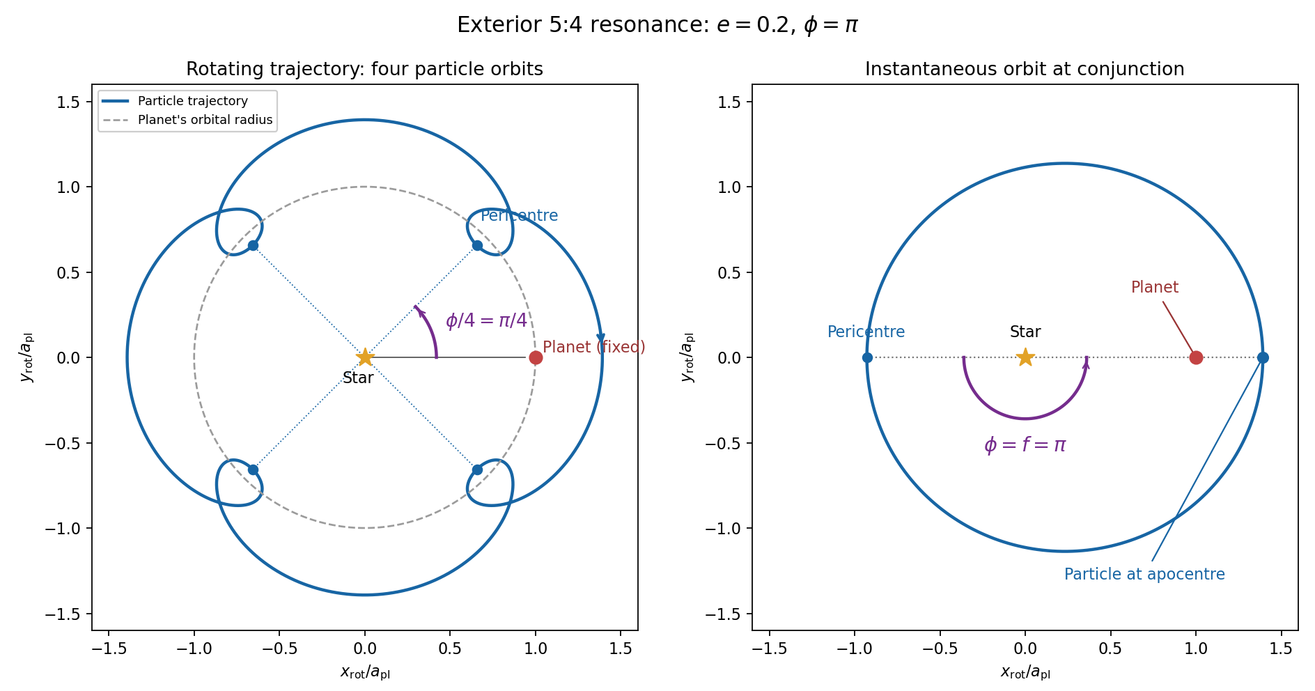
For the evolution equations, $\lambda$ must be the mean longitude. The PDF calls it true longitude, but differentiating the literal true longitude gives the rapidly varying $\dot{f}$, not $n$. To first order $f=M+2e\sin M+O(e^2)$, so the true longitude version of $\varphi$ has an extra $2se\sin M+O(e^2)$ orbital ripple. The stated Lagrange planetary equations and slow complex eccentricity equation are interpreted consistently as orbit-averaged equations in mean longitude. The pericentre geometry of an exterior resonance above is unchanged by this distinction.

Let $F_r,F_{\theta }$ be perturbing forces, and let $m$ be the particle's mass. The angular momentum about the star satisfiesThe central gravitational force and the radial perturbation have zero torque. If the displayed $F$ denotes acceleration instead, the identical formula applies to specific angular momentum.

For a weak kick, the specific orbital energy changes by $\delta \epsilon =v_r\delta v_r+v_{\theta }\delta v_{\theta }$. A planet leading the particle pulls it forwards, while a trailing planet pulls it backwards. For a nearly circular exterior Kepler orbit, a forward tangential kick raises angular momentum and semi-major axis, lowers mean motion, and makes the next conjunction occur sooner in the synodic cycle. Its longitude retreats relative to the unperturbed conjunction sequence. A backward kick produces the opposite shift. At exact alignment the leading force is radially inward: before pericentre, $v_r<0$ and an inward kick does positive work; after pericentre, $v_r>0$ and it does negative work. These likewise raise or lower semi-major axis. At an apsis, a purely radial infinitesimal kick has no first-order energy change but changes the eccentricity vector, so angular momentum alone does not determine every timing change.

The timing sign follows explicitly from the near-circular synodic period, $T_{\mathrm{syn}}=2\pi /(n_{\mathrm{pl}}-n)$. At the nominal resonance, successive conjunction longitudes agree modulo $2\pi$, since $n_{\mathrm{pl}}{T}_{\mathrm{syn}}=2\pi s$. A persistent small change givesThis is the accumulated mean timing shift; an actual impulsive encounter can also change the instantaneous orbital phase and longitude of periapsis.

Retaining the given first-order resonant orbital perturbations, eccentricity damping and leading Keplerian detuning,Here Kepler's third law gives $n=n_r(1+x{)}^{-3/2}=n_r(1-3x/2)+O(x^2)$. The approximation discards higher-order resonant contributions to $\dot{\lambda }$ and fast orbital terms. Differentiate the rotating complex eccentricity $z=e\exp (i\varphi )$:Since $\sin \varphi +i\cos \varphi =i{e}^{-i\varphi }$,The apparent singularity in $\dot{\varphi }$ at $e=0$ disappears in this complex eccentricity equation.

Take $A>0$, and the conventional positive resonant coefficient $C>0$. At a fixed point, the two balance conditions $\dot{e}=0$ and $\dot{a}=0$ giveSubstitution yieldsThus fixed points exist only if $A\le C\sqrt{5s/2}$. With strict inequality, put $S=\sqrt{(5/2)s{C}^2-A^2}$ and ${\psi }_f=\arctan (A/S)\in (0,\pi /2)$. Thenrespectively. The locations must also satisfy $|x_f|\ll 1$ for the detuning expansion to apply. At equality the phases merge at $3\pi /2$ and $x_f=0$. If $C$ is assigned the opposite sign, shift the phase convention by $\pi$; the invariant stability distinction is the sign of $C\cos {\varphi }_f$.

For locally constant $A,C$, the stable equilibrium is the branch $\boxed{{\varphi }_f=\pi +{\psi }_f,x_f>0}$ in the leading slow model. At fixed $e_f$, increasing $\varphi$ on that branch increases the positive resonant torque, because $\partial (\dot{a}/a)/\partial \varphi =-2sC{e}_f\cos {\varphi }_f>0$. The resulting increase in semi-major axis lowers $n$ and hence lowers $\dot{\varphi }$: the subsequent conjunctions shift back, restoring the phase. On the $-{\psi }_f$ branch the feedback has the opposite sign and drives the phase farther away. Eccentricity damping removes the oscillatory disturbance on the restoring branch.

One can verify that this feedback stabilizes the coupled variables rather than just the phase. Treat $A,C$ as locally constant, and write $z=u+iv$. Then $\dot{u}=-Au+Bxv$, $\dot{v}=-C-Av-Bxu$ and $\dot{x}\simeq -2sCv-4A/5$. At a fixed point $Bxv=Au$. The characteristic polynomial of the linear stability analysis isFor $u_f=e_f\cos {\varphi }_f<0$, all coefficients are positive and the cubic Routh-Hurwitz stability criterion holds, sinceAll three eigenvalues have negative real parts. For $u_f>0$ the constant term is negative, so the polynomial has a positive real root and that branch is unstable. The merged case has a zero eigenvalue. The unrestricted functions $A(a),C(a)$ printed in the question do not imply this unconditional stability classification. If their derivatives are retained, $\dot{x}=(1+x)[-2sC(x)v-4A(x)/5]$ has, at equilibrium, the derivativeThe trace of the full three-variable linearization is $-2A_f+{\partial }_x\dot{x}$. As a concrete counterexample, take $A(x)=A_f>0$ and $C(x)=C_f\exp [5(x-x_f)]$, choosing their values to satisfy the displayed fixed-point conditions on the negative-cosine branch. Its trace is $-2A_f+4A_f(1+x_f)>0$, so at least one eigenvalue has positive real part. Both coefficients are smooth. Thus the restoring conjunction feedback identifies the stable branch of the usual locally constant model, but additional assumptions on coefficient variation are necessary to assert stability for every allowed function.

Inversion in a circle of center $c$ and radius $R$ is $K(z)=c+R^2/(\bar{z}-\bar{c})$ on the extended plane. It sends infinity to $c$, so it interchanges zero and infinity exactly when $c=0$.

For the unit-circle inversion $J$, both $J$ and $K$ are involutions. If $KJ{z}_0=z_0$, applying $K$ gives $J{z}_0=K{z}_0$. Writing $w=J{z}_0$, we have $Jw=z_0$ and $Kw=z_0$, and therefore $KJw=K{z}_0=w$. This proves both assertions about the fixed points.

We now show that one fixed point is inside the disk and use it as the hyperbolic center. Rotate coordinates to make the Euclidean center $c=a\ge 0$. The hypothesis is $a+R<1$. If $a=0$ the conclusion follows immediately from the radial hyperbolic distance. If $a>0$, thenfor its fixed points. Since $1+a^2-R^2>2a$, this quadratic has two positive roots with product one, one $p\in (0,1)$ and the other $1/p>1$.

The disk automorphism $h(z)=(z-p)/(1-pz)$ is a Poincare disc automorphism. It sends the two fixed points to zero and infinity and commutes with $J$ on the extended plane. Consequently $K^{\prime }=hK{h}^{-1}=(hT{h}^{-1})J$ interchanges zero and infinity. Conjugation takes circle inversion to inversion in the image circle, so the first part says that $h(\Gamma )$ is centered at zero. Its Euclidean radius is some $s<1$.

In the Poincaré disk metric, integrating the radial length element givesSince $h$ preserves distance, the original circle is exactlyUndoing the preliminary rotation gives the center for arbitrary complex $c$.

This identifies the hyperbolic circle in the Poincare disc intrinsically.

The positive steady state satisfies $1+b(N^{\ast }{)}^2=r$, soWith $N_t=N^{\ast }+{\eta }_t$, the linearization isIts characteristic polynomial is ${\lambda }^2-\lambda +d$, where $d=2(r-1)/r$. The roots are inside the unit disk precisely when $0<d<1$: when they are real they are positive with sum one, and when complex conjugate their common modulus is $\sqrt{d}$. Therefore the fixed point is linearly asymptotically stable for $1<r<2$ and unstable for $r>2$. At $r=2$,This proves period six for the neutral linearized oscillations. The stronger printed claim of a nonlinear period-six branch is not valid for the stated recurrence. It is important to distinguish these two assertions.

Here is a local obstruction, which also checks that the qualification is not merely absence of a proof. Normalize by the moving fixed point, let $x=N_{t-1}/N^{\ast }(r)-1$, $y=N_t/N^{\ast }(r)-1$, and definePut $v=(x,y{)}^T$, $\delta =r-2$, and $Q=x^2-xy+y^2>0$ for $v\ne 0$. The quadratic and cubic terms of $F_2$'s second component are $x^2/2-xy+x^{2}y/2$. Composing six times givesIn particular the quadratic terms cancel, while the cubic components are $-(x+2y)Q/2$ and $(2x-3y)Q/2$. If a small nonzero $v$ were a period-six point, invertibility of $B$ and the norm of this equation would imply $|\delta |=O(|v{|}^2)$. Taking its determinant with $Bv$ then givesSince $Q\ge |v{|}^2/2$, this is impossible for sufficiently small nonzero $v$. Thus no nontrivial nonlinear six-cycle bifurcates locally at $r=2$. At the threshold the same expansion gives $Q(F_2^6(v))=Q(v)-2Q(v{)}^2+O(|v{|}^5)$, so the fixed point is actually locally asymptotically stable nonlinearly, with slow decay. The valid intended linear-stability conclusion is the period-six neutral oscillation above; a literal nonlinear assertion requires a changed model or wording. This is an example of the distinction between linear resonance and nonlinear periodic bifurcation.

The nullclines are $y=\mu x$ and $y=x^2/[\nu (1+x^2)]$. At a nonzero fixed point, cancellation of $x$ yields $\mu \nu =x/(1+x^2)$. The latter function attains its maximum $1/2$ at $x=1$. HenceFor $0<\mu <{\mu }_c$, $x_{-}<1<x_{+}$ and $x_{-}{x}_{+}=1$.

The Jacobian matrix isAt $O$ the distinct eigenvalues are $-\mu ,-\nu$, so the origin is a stable node. At a nonzero fixed point its trace is $-(\mu +\nu )<0$ andThe discriminant is $(\mu -\nu {)}^2+8x/(1+x^2{)}^2>0$. Thus $P_{-}$ is a saddle and $P_{+}$ is a stable node, never a focus.

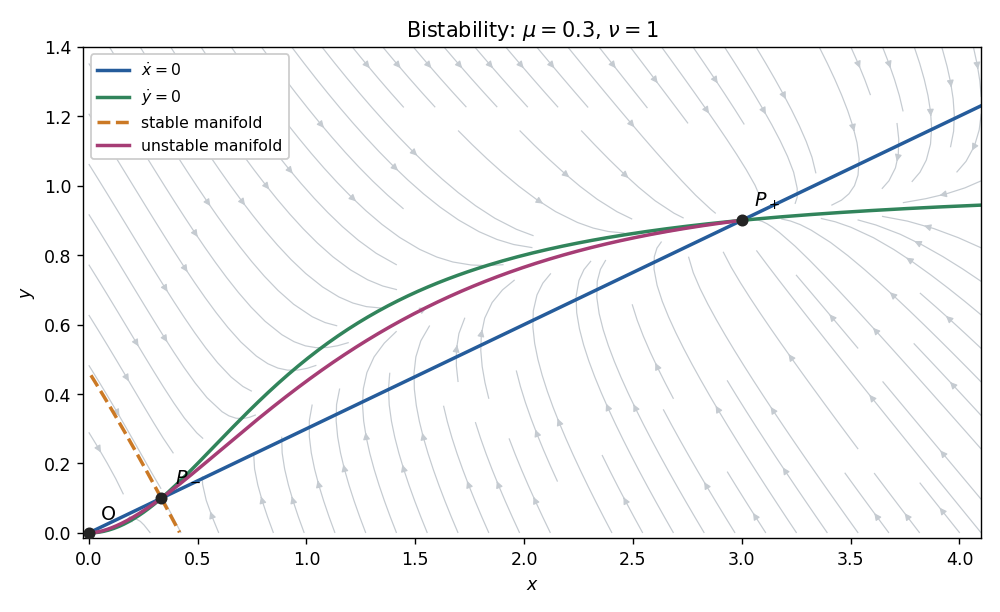
Above the straight nullcline $\dot{x}>0$; below it $\dot{x}<0$. Below the curved nullcline $\dot{y}>0$; above it $\dot{y}<0$. At the saddle, an eigenvector can be chosen as $(1,\mu +\lambda )$: the stable eigenvalue gives negative slope, and the unstable eigenvalue gives positive slope. The stable manifold is the basin boundary. The two branches of the unstable manifold lead respectively to the origin and the positive stable node, as illustrated for representative parameters.

The nonnegative quadrant is forward invariant. Since $\dot{y}\le 1-\nu y$, $y$ stays bounded, and then $\dot{x}=-\mu x+y$ also bounds $x$. Moreover the divergence is the negative constant $-(\mu +\nu )$, excluding periodic or homoclinic loops by the Bendixson-Dulac criterion. The Poincaré-Bendixson theorem then leaves convergence to a fixed point. Initial data on the saddle's stable manifold approach the saddle; data in the two open basins approach extinction at $O$ or persistence at $P_{+}$, respectively.

Fix $z$ with $|z|<1-\epsilon$, and let $\Pi (w)=w/\max (1,|w|)$ be radial projection to the closed disc. The continuous map $p\mapsto \Pi (p-G(p)+z)$ has a fixed point $p$ by the Brouwer fixed-point theorem. On the boundary, $|p-G(p)+z|<\epsilon +|z|<1$, so its image under $\Pi$ is interior and cannot equal the boundary point $p$. Therefore $p\in B$. An interior fixed point of this projection must satisfy $p-G(p)+z=p$, because points outside the disc project to its boundary. Thus $G(p)=z$. Every $z\in B_{1-\epsilon }(0)$ belongs to $G(B)$.

Suppose first that a retraction $R:D\to C$ exists. The continuous map $p\mapsto -R(p)$ takes $D$ to itself, so the Brouwer fixed-point theorem gives $p=-R(p)$. Such $p$ lies on $C$, where $R(p)=p$, contradicting $p=-p$.

Conversely, suppose a continuous map $T:D\to D$ has no fixed point. For each $p$, follow the ray from $T(p)$ through $p$ to its last intersection with $C$. This defines a retraction. More explicitly, put $a=p-T(p)\ne 0$ and setThe positive-root formula is continuous, $t(p)\ge 1$, and $R(p)$ is on the unit circle. If $p\in C$, the last intersection is $p$ itself, so $R(p)=p$. Thus the nonexistence of a retraction rules out a fixed-point-free $T$, proving the equivalence.

The planar Brouwer fixed-point theorem states that every continuous map from a closed disc to itself has a fixed point.