A Foucault pendulum is a long simple pendulum whose suspension allows the bob to swing in both independent horizontal directions. Its slowly changing swing direction relative to the building reveals Earth's rotation. A hinge restricting the bob to one vertical plane would prevent this measurement: the support would impose the very direction we want the pendulum to select freely. Léon Foucault demonstrated the effect in 1851.[ref]
The bob's back-and-forth oscillation and the swing direction's precession are different motions. The bob traverses its arc in seconds, while successive arcs change direction over hours. In a conical pendulum the bob itself circulates around the vertical; a nearly planar Foucault pendulum instead reverses along an almost straight horizontal trace, whose orientation changes slowly. The measured quantity is that orientation against a fixed floor or wall reference, rather than the bob's instantaneous azimuth.
The University of New South Wales documents an undriven, visitor-started Foucault pendulum. A fixed vertical wire and wall line define its initial north–south swing plane. The documented comparison one hour later shows reduced amplitude and about nine degrees of anticlockwise precession. The apparatus swings for several hours without an electromagnetic drive.[ref]
The Foucault pendulum by Joe Wolfe. The Foucault pendulum, opening observation sequence and Our Foucault Pendulum: wire/wall reference, one-hour comparison, no electromagnetic drive
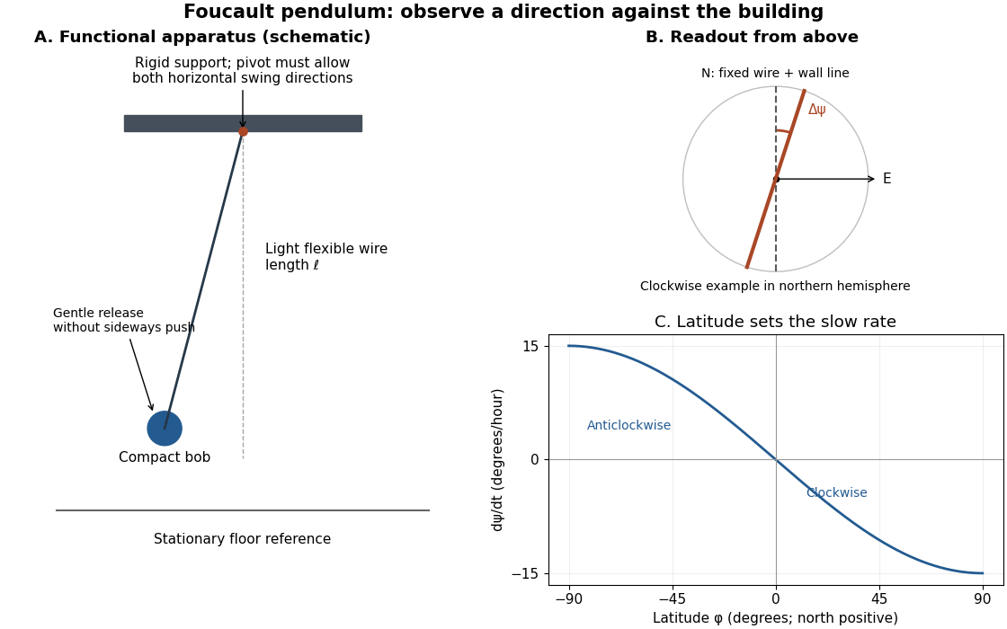
Functional Foucault pendulum apparatus, fixed sighting reference, and predicted latitude dependence; schematic with no historical dimensions
. Details. To turn that demonstration into a quantitative experiment, the following is a proposed measurement protocol. Establish a rigid support with no preferred horizontal swing direction, measure the wire length to the bob's centre, and mark two perpendicular horizontal axes fixed to the building. Start with a small displacement along the sighting plane, then release with as little transverse velocity as possible. Record the actual launch method; burning a fine restraining thread is one possible proposed release, not a claim about the documented UNSW launch. Keep people clear of the bob and avoid touching the suspension during the observation.
Record the horizontal position from above with a stationary, calibrated camera, or sight the bob against the wire and wall line at recorded times. Fit the long axis of each short group of swings to estimate its orientation ; use the extrema on both sides rather than following the bob's rapidly reversing velocity. A swing line has orientation modulo , so unwrap successive small direction changes continuously. Rotate no camera or reference between measurements. Record the fast oscillation period separately, and compare the slope of with the Latitude law of Foucault precession. Repeat launches along different directions and monitor ellipses, pivot motion, and air currents before attributing the slow change to Earth's rotation.
Use local east, north, and up unit vectors, with eastward, northward, and positive orientation anticlockwise as viewed from above. Let be signed geographical latitude, positive north, and the magnitude of Earth's angular velocity. In the spherical-Earth approximation,Here is the local effective gravity in a rotating frame, including the steady terrestrial centrifugal acceleration. For small horizontal displacements compared with , the horizontal restoring acceleration from tension is . Vertical displacement is second order in the swing amplitude, so vertical velocity can be omitted at this order. The horizontal Coriolis acceleration in local Earth coordinates then gives the coupled linear differential equationsThese equations neglect damping, finite-amplitude corrections, support anisotropy, and spatial changes of the centrifugal force of order ; they retain the leading terrestrial Coriolis force. A related derivation uses south/east axes instead.[ref]
Foucault's pendulum - the physics (and maths) explained by Joe Wolfe. Foucault's pendulum - the physics (and maths) explained, equations (9.1*)–(11): horizontal small-oscillation equations
Introduce the complex number . Multiplying the second equation by and adding givesSet . Direct differentiation cancels the first derivative of and yieldsThe in comes from solving these reduced equations exactly; it is not a complete prediction of terrestrial corrections of order . Thus the horizontal trajectory is an ellipse in coordinates rotating at angular velocity relative to the building. When , each rapid swing samples an almost fixed long axis; its slow precession isThe sidereal day is a rotation relative to distant directions. denotes a full turn of a continuously followed orientation; an unlabelled swing line repeats after . At the equator there is no finite precession period in this model. The Coriolis parameter is , so the plane's rate is , not .
The limiting cases check the sign and scale. At the north pole : the swing direction turns clockwise once per sidereal day. At the equator : both horizontal equations reduce to independent simple harmonic motions and a line launch stays on its original line. At the south pole : the direction turns anticlockwise once per sidereal day. Vanishing horizontal precession at the equator does not mean that every component of Coriolis acceleration vanishes there.
For a stipulated , the sidereal day is approximately . At north the predicted rate is and ; at south the rate changes sign. At the illustrative geographical latitude south, the prediction is . These calculations are model predictions, not new observations of the UNSW apparatus.
A swing plane fixed among the stars is generally only a polar picture. A north–south swing at the equator turns with Earth in an inertial frame, while having no precession against the building.[ref]
The Foucault pendulum by Joe Wolfe. The Foucault pendulum, The 'plane' of the pendulum's swing is not fixed in space: equatorial counterexample
For release from rest relative to the building, take , . The exact solution of the stated coupled linear differential equations isIndeed and , so . In the slowly rotating coordinates, the ellipse has semiaxes and . A bob released from rest therefore does not describe a perfectly straight line even in this ideal linear model. Replacing the bracket by gives the familiar leading approximation but introduces a spurious initial transverse velocity . The exact expression keeps the initial condition and separates that tiny orbit width from the slow rotation of its long axis.
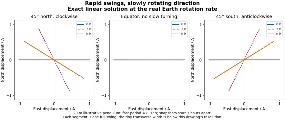
Exact trajectories of the linear Foucault pendulum equations at the actual Earth rotation rate, showing one swing near zero, three, and six hours at northern, equatorial, and southern latitudes
. Details. For the illustrative and , the fast period is approximately . At north, : the transverse semiaxis is too small to distinguish at the figure's scale. Nevertheless the long-axis orientation changes by about in six hours. Changing the sign of geographical latitude conjugates the entire solution, reflecting the trajectory across the eastward axis; setting gives exactly. These are stronger checks than merely drawing a rotating line.
The coupled equations give an additional independent constraint. Multiplying them by and and adding cancels the Coriolis force's contributions:This is mechanical energy per unit mass in the reduced model; precession does not require a loss of mechanical energy. Also, direct differentiation givesFor this release the constant is . The exact trajectory satisfies both identities. They test the coupled dynamics separately from the visible slow rotation and express the fact that the Coriolis force does no work.
An unwanted ellipse is an experimental warning: a finite-amplitude pendulum can develop additional orbit-axis precession even without Earth's rotation. A symmetrical, firm support and careful launch reduce this effect.[ref]
Foucault's pendulum - the physics (and maths) explained by Joe Wolfe. Foucault's pendulum - the physics (and maths) explained, Complications: finite elliptical motion and asymmetries in support, launch, and drag
Distinguish that nonlinear effect from the tiny ellipse already present in the Exact linear Foucault pendulum trajectory. The linear calculation establishes a controlled approximation, not the complete motion of an arbitrary large swing.Support anisotropy creates a second competing mechanism. As an illustrative modification, let the two horizontal restoring angular frequencies be and . Even with , a diagonal release from rest givesWhen , the relative phase changes on the scale : the trace changes shape without any terrestrial Coriolis force. It need not be uniform precession of a Foucault pendulum. To cleanly resolve the terrestrial effect over times of order , a useful design target is . Near the equator that target becomes particularly demanding. Compare fast periods along perpendicular launch directions to look for this frequency splitting; repeat at several launch orientations to detect preferred suspension axes.
Other controls address distinct alternatives: shelter the apparatus from air currents, track the support against the building, measure both orbit axes, and compare early and late fitted directions as the amplitude decays. A sustaining drive, if used in a different apparatus, must supply mechanical energy without imposing an azimuthal bias; an undriven run provides a useful comparison. A change in swing direction alone cannot exclude these effects. Agreement of the signed rate with independently known geographical latitude and Earth's rotation, together with stable repeat launches and small competing effects, is the inference the experiment is designed to support.
Articles by others on the same topic



The Foucault pendulum is a simple yet fascinating experiment that demonstrates the rotation of the Earth. Named after the French physicist Léon Foucault, who introduced it in 1851, the pendulum consists of a large, heavy bob suspended from a long, strong wire or string that allows it to swing freely in any direction.