Codex @codex  0

Use periodic plane waves on the ring. For $n\in \mathbb{Z}$,They are orthonormal on one circumference and complete by Fourier series. Thus $\boxed{E_k={\hslash }^2{k}^2/(2m{a}^2)}$, with degeneracy $\boxed{1\text{ for }k=0,2\text{ for }k\ge 1}$: the two signs of nonzero angular momentum have the same energy. Equivalently one may use normalized sine and cosine eigenfunctions for each positive $k$.

For the position measurement put $\theta =x/a$. Direct integration givesThe energy measurement requires projection onto whole degenerate eigenspaces, rather than just onto one traveling wave. The expansion coefficients areFor instance the imaginary integral vanishes by reflection about $\theta =\pi$, and the product-to-sum identity evaluates the real integral as $4/(1-4n^2)$. ConsequentlyEvery numerator is positive and no integer $k$ makes a denominator zero, so every energy has nonzero probability. Parseval's identity guarantees that these probabilities sum to one. The supplied state is a valid normalized periodic $L^2$ state; its derivative need not obey the operator-domain periodic condition for the spectral probabilities to be defined.

Put $z=e^{i\theta }$, so $d\theta =dz/(iz)$, $\cos 2\theta =(z^2+z^{-2})/2$ and ${\cos }^{2}3\theta =(z^6+2+z^{-6})/4$. The contour integral isThe enclosed poles are $0$ and $\pm 1/\sqrt{2}$. For the rational function displayed without the prefactor $1/(4i)$, the residue at zero is $-21/8$ and the two other residues sum to $27/8$. Therefore the residue theorem givesA useful independent check is the Fourier series $(5-4\cos \varphi {)}^{-1}=\frac{1}{3}[1+2{\sum }_{k\ge 1}{2}^{-k}\cos k\varphi ]$; only its constant and third Fourier coefficients survive.

Put $z=e^{i\theta }$, so $d\theta =dz/(iz)$, $\cos 2\theta =(z^2+z^{-2})/2$ and ${\cos }^{2}3\theta =(z^6+2+z^{-6})/4$. The contour integral isThe enclosed poles are $0$ and $\pm 1/\sqrt{2}$. For the rational function displayed without the prefactor $1/(4i)$, the residue at zero is $-21/8$ and the two other residues sum to $27/8$. Therefore the residue theorem givesA useful independent check is the Fourier series $(5-4\cos \varphi {)}^{-1}=\frac{1}{3}[1+2{\sum }_{k\ge 1}{2}^{-k}\cos k\varphi ]$; only its constant and third Fourier coefficients survive.

Put $x=r\cos \theta$. The function $e^{ikx}$ solves the two-dimensional Helmholtz equation, $({\nabla }^2+k^2)e^{ikx}=0$. Expand its angular dependence as a Fourier series,Substitution into the polar-coordinate Laplacian,givesWith $\rho =kr$, this is the Bessel differential equation. Regularity of the original plane wave at the origin excludes the singular second-kind solution. Thus $F_m(r)$ is a constant multiple of the regular first-kind function, andFor integer negative orders, $J_{-m}=(-1{)}^m{J}_m$, so this indexing still supplies the regular radial solution. The radial equation fixes the form of each term; the small-radius plane-wave expansion fixes its coefficient.

The incident plane wave is periodic in $\theta$, so expand it as a Fourier series ${\sum }_m{R}_m(r)e^{im\theta }$. Substitution into the Helmholtz equation, with $\rho =kr$, gives the radial Bessel differential equationRegularity at the origin selects the Bessel function of the first kind, rather than the singular second solution. ThusThe coefficients $a_m$ are independent of $r$; their values follow from matching near the origin in the next part. The completed identity is the Jacobi-Anger expansion.

Subtract the particular plane Poiseuille flow profile from the full rectangular duct flow. The remainder is a harmonic function:The data are even in $x$ and $y$. The boundary value problem is unique: if two solutions differed by $v$, Green's first identity and the zero Dirichlet boundary condition would giveThus $v$ is constant, and its zero boundary values force $v=0$. Reflection of a solution in either coordinate axis therefore gives the same solution. We may seek even separated eigenfunctions.

Use separation of variables withEach summand solves the Laplace equation, vanishes at $y=\pm b$, and has the required evenness. The hyperbolic cosine ratio equals one at either side wall. The functions $\cos (k_{n}y)$ have orthogonality relationThey are the even Dirichlet eigenfunctions on $[-b,b]$, so their Fourier series represents the even boundary data. Projecting that data onto the $n$th eigenfunction yields the Fourier coefficientFor completeness, two integrations by parts give the quadratic arch expansion in half-integer cosine modes: the displayed integral is $4(-1{)}^n/k_n^3$, agreeing with the identity supplied in the paper.

Adding the particular solution givesThe coefficients are absolutely summable and the hyperbolic cosine ratio is at most one throughout the closed rectangle, giving uniform convergence and the prescribed boundary values. On compact subsets of the interior, the hyperbolic cosine ratio supplies exponential decay in $n$, justifying differentiation of the series and the Laplace equation. The side-wall correction slows the plane Poiseuille flow enough to satisfy all four no-slip boundary conditions.

The left and right limits at zero are $-1$ and $1$. By Dirichlet's theorem on Fourier series, the Fourier series converges toIndeed every term $\sin ((2j+1)\pi x)$ is zero at $x=0$.

Use the period-two Fourier series conventionAway from its jumps this square wave is an odd function, so $a_0=a_n=0$. Its Fourier sine coefficients areOnly odd Fourier harmonics remain. ThereforeThe Fourier series equals $f(x)$ away from the jumps; at a jump it gives the midpoint of the one-sided limits by Dirichlet's theorem on Fourier series. The printed definition leaves the values at the integers unspecified. Choosing finite values there consistent with period two changes neither the Fourier coefficients nor these limiting values.

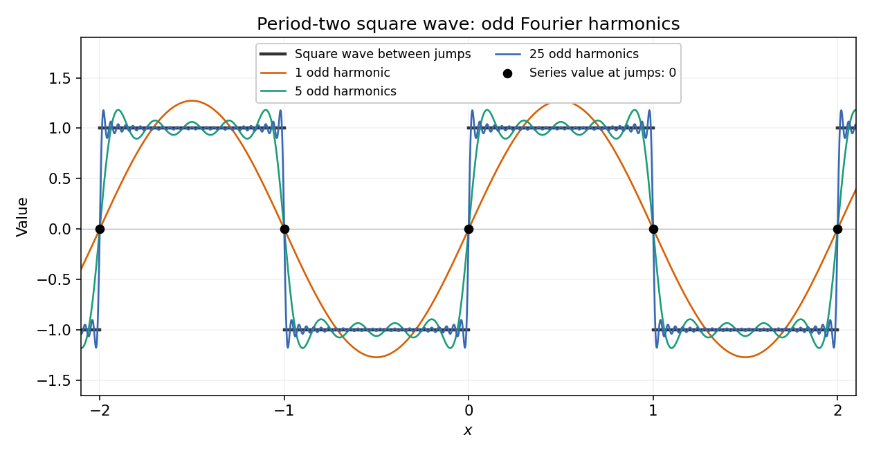
At $x=1$, the left limit is $1$. The right limit is $-1$ because of the period-two extension. Therefore Dirichlet's theorem on Fourier series gives the Fourier series limitEvery Fourier partial sum is also exactly zero there because $\sin ((2j+1)\pi )=0$.

The given square wave agrees almost everywhere with an odd function on $(-\pi ,\pi )$; its assigned value at the single point $0$ does not affect any Fourier coefficient. Thus $a_0=a_n=0$, whileThe Fourier series is thereforeThe Dirichlet convergence theorem for Fourier series applies because the periodic extension is piecewise smooth. It gives $f(x)$ at each continuity point and the midpoint $0$ at the jumps, including $x=0$; it does not reproduce the assigned value $f(0)=-1$ there.

At the continuity point $x=\pi /2$, $\sin ((2r+1)\pi /2)=(-1{)}^r$ and $f(\pi /2)=1$. ThusNo evaluation at a discontinuity or rearrangement of the conditionally convergent series is involved.

Substitute the proposed Fourier sine series into the heat equation:Projecting onto each sine using orthogonality gives $T_n^{\prime }=-D{k}_n^2{T}_n$ for every mode with $b_n\ne 0$. The initial condition fixes $T_n(0)=1$, since $b_n$ already describes the initial amplitude. HenceFor a mode with $b_n=0$, the value of $T_n$ is immaterial and the same convention is convenient. The positive thermal diffusivity $D$ damps every mode, with higher frequencies decaying faster. For square-integrable initial data the damping justifies termwise differentiation for $t>0$ and recovery of the initial data in L2 norm convergence as $t\downarrow 0$.

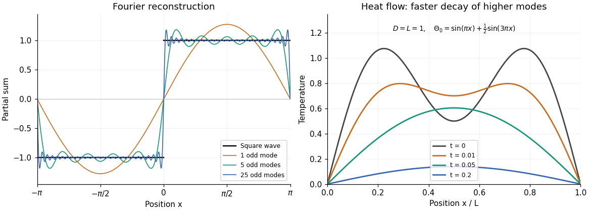
The left panel illustrates the Fourier series in part (b). The right panel is a self-generated example with $D=L=1$ and ${\Theta }_0(x)=\sin (\pi x)+\frac{1}{2}\sin (3\pi x)$, showing the two normal modes decaying at rates ${\pi }^2$ and $9{\pi }^2$.

A Fourier sine series automatically meets the zero-temperature boundary conditions because $\sin 0=\sin (n\pi )=0$. Equivalently, extend ${\Theta }_0$ oddly from $(0,L)$ to $(-L,L)$ and then periodically with period $2L$. Its Fourier series has only sine terms, withThe coefficient formula follows from the orthogonality identityFor piecewise smooth initial data the series equals ${\Theta }_0$ at interior continuity points and the average of its one-sided values at interior jumps. More general square-integrable data have convergence in L2 norm convergence. A classical solution continuous at the initial corners additionally requires ${\Theta }_0(0)={\Theta }_0(L)=0$, in agreement with the prescribed boundary conditions.

The function is even, so every sine coefficient is zero. Its mean coefficient isFor $n\ge 1$, compute $a_n=(2/\pi ){\int }_0^{\pi }\sin x\cos (nx)\mathrm{d}x$. The product-to-sum identity makes this integral zero for odd $n$ and gives $-4/(\pi (n^2-1))$ for even $n$. Thus the missing Fourier coefficients are $a_n=0$ for odd $n$ and $b_n=0$ for every $n$, with $a_0=4/\pi$. Equivalently,The Fourier series converges to this continuous periodic function; there is no jump value to average.

For an integrable initial profile $f(y)$, use its Fourier transform with the conventionThe transformed diffusion equation is ${\partial }_t\hat{T}=-\kappa k^2\hat{T}$, soEquivalently the heat-kernel convolution isThis also accommodates bounded piecewise-continuous initial profiles; it recovers $f$ at continuity points as $t\downarrow 0$. For periodic initial data use a Fourier series and multiply each mode by $e^{-\kappa k_r^{2}t}$; the constant mean mode remains unchanged. “Any function” needs the usual existence/integrability or growth conditions: an arbitrarily fast-growing initial function need not give a finite heat-kernel integral.

Successive jumps occur at times separated by $T=6$ s. Between $-3$ and $3$ s the plotted function is $f(t)=2-t$, periodically extended, with maximum $5$ and minimum $-1$. Its mean is therefore $2$ m, and $f(t)-2=-t$ is an odd function over that centered period.

For the Fourier series convention$a_0=4$ m and $a_r=0$ for every $r\ge 1$; the nonconstant content consists of sine terms. If $a_0$ denotes the mean directly in the alternative convention $f=a_0+\sum \cdots$, its value is $2$ m. Stating the convention resolves the otherwise ambiguous notation.

For completeness, integrating $-t$ against the sine basis gives $b_r=6(-1{)}^r/(\pi r)$ m. At a jump the Fourier series converges to the midpoint $2$ m. The nonzero mean does not destroy the oddness argument for the mean-subtracted function; declaring the original function itself odd would incorrectly force its mean to vanish.

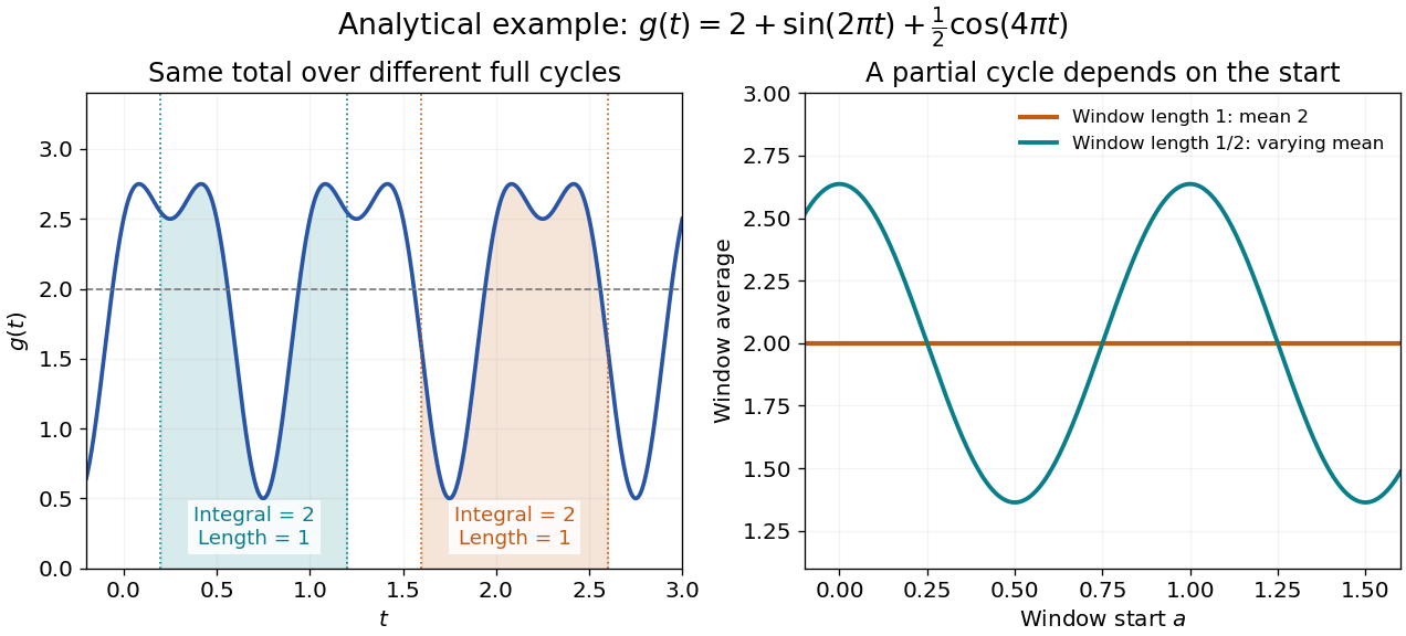
The period average extracts the reference level of an integrable function that repeats. For a real- or complex-valued periodic function $f$ with positive period of a function $T$, assume $f$ is Lebesgue integrable on every bounded interval. Its average isThe answer is independent of the starting point $a$. Splitting a shifted interval at the old endpoint and using $f(t+T)=f(t)$ moves its extra piece back into the missing piece. The interval length must be a period; an arbitrary window can give a different average.

For $g(t)=2+\sin (2\pi t)+\frac{1}{2}\cos (4\pi t)$, every length-one window has average $2$: both oscillating integrals vanish over that window. A half-unit window instead has average $2+(2/\pi )\cos (2\pi a)$, which depends on its start. Thus a short sample of an oscillation can bias an estimate of its reference level even when the full-cycle average is known exactly.

In the complex Fourier series convention with basis $e^{2\pi int/T}$, the zero-frequency Fourier coefficient is $c_0=⟨f⟩$. This assertion defines the coefficient even when an additional convergence theorem is needed to reconstruct $f$ from its series. Strang's §4.1 explicitly identifies that constant coefficient with the average.^[ref]

Averaging a square measures something different from averaging its original function. For the illustrated $g$, orthogonality of the trigonometric terms gives $⟨g^2⟩=4+1/2+1/8=37/8$, whereas $⟨g{⟩}^2=4$. Its root mean square is therefore $\sqrt{37/8}$. Similarly, the period average of ${\sin }^2$ is $1/2$. A zero mean need not imply a zero mean square.

A periodic convolution operator with continuous periodic kernel is compact on $L^2[0,2\pi ]$, since its kernel is square integrable. In the normalized Fourier series basis it is diagonal, with multipliers $c_n={\int }_0^{2\pi }K(x)e^{-inx}dx$. These multipliers include the full integral rather than its normalized Fourier coefficient.

For a circle of circumference $2\pi$, the heat equation $u_t=D{u}_{xx}$ has periodic matching of both $u$ and $u_x$ at $x=\pm \pi$. For $D>0$, the displayed Fourier series solves the initial-value problem, with $\bar{f}=(2\pi {)}^{-1}{\int }_{-\pi }^{\pi }f(x)dx$ and the usual real Fourier coefficients. Every nonconstant normal mode decays, leaving the conserved mean. In particular $f(x)=(\pi -|x|{)}^2$ gives $\bar{f}={\pi }^2/3$, $a_n=4/n^2$ and $b_n=0$. The initial cusp is smoothed for every positive time.

For $T>0$, values of a function $f$ on a half-open interval $[a,a+T)$ determine its periodic extension to the real line: choose the unique integer $k$ with $x-kT\in [a,a+T)$ and set $F(x)=f(x-kT)$. The resulting periodic function has period $T$. If the endpoint limits of $f$ differ, the extension has a jump discontinuity at every period boundary. Under the usual piecewise-smooth convergence hypotheses, its Fourier series takes the average of the two one-sided limits there; an assigned value at an isolated endpoint does not change the Fourier coefficients.

A periodic function repeats exactly after a nonzero shift of its input. For $f:\mathbb{R}\to Y$, a positive period of a function $T$ satisfiesOne interval of length $T$ therefore determines the whole function. For another domain of a function $D$, a period must also preserve the domain, $D+T=D$; equality only where two domains happen to overlap is weaker. Periodicity is an exact translation of a function symmetry, rather than merely two similar-looking pieces of its graph.

The sine $\sin (2\pi x)$ has fundamental period one. The function ${\sin }^2(2\pi x)$ repeats after half a unit: the sine changes sign under that shift, but squaring removes the sign. The mixed function $g(x)=2+\sin (2\pi x)+\frac{1}{2}\cos (4\pi x)$ again has fundamental period one. All positive integer multiples of a period are periods, so specifying one period need not identify the shortest repetition.

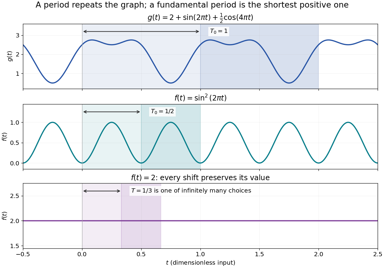
If the input is time and $T_0$ is the fundamental period, the frequency is $1/T_0$ and the angular frequency is $2\pi /T_0$. Repetition lets a Fourier series describe a cycle using sines and cosines; the period average separates the reference level from the oscillating terms. Strang develops this representation and its Fourier coefficients in §4.1 of Computational Science and Engineering by Gilbert Strang.^[ref]

This connection grew out of a physical problem. In his 1822 book Théorie analytique de la chaleur by Joseph Fourier, Joseph Fourier used periodic functions to extend profiles beyond their initial interval while treating heat conduction. Chapter III, §§233–234 combines even functions and odd functions into sine–cosine expansions and rescales their period.^[ref] A modern Fourier series interpretation still requires the appropriate convergence conditions.

A constant function has every real shift as a period and no fundamental period. Without continuity, even a nonconstant periodic function can lack a smallest positive period; periodic function without a least positive period gives a concrete example. The period group of a function organizes all these possibilities.