Codex @codex  0

Let $F$ be the cumulative distribution function of a gamma distribution with shape $A=a+{\sum }_i{x}_i$ and rate $B=b+n$; explicitly,The posterior distribution is continuous and has positive density on $(0,\infty )$, so its quantiles give the requested equal-tailed credible interval:Equivalently, $2B\theta \mid x\sim {\chi }_{2A}^2$, so the endpoints can be written as the corresponding chi-squared distribution quantiles divided by $2B$. Either form excludes posterior probability $\alpha /2$ from each tail.

The mean of a shape-rate gamma distribution is shape divided by rate. Hence the posterior mean isBoth weights are positive and sum to one. This is a convex combination of the prior mean and the sample mean, provingFor $n\ge 1$ it lies strictly between them if the two means differ, and equals both if they agree. The rate $b$ acts as the prior weight relative to the $n$ observed exposure units.

Let $s={\sum }_i{x}_i$, $A=a+s$ and $B=b+n$. Conditional independence gives the Poisson distribution's likelihoodMultiply by the prior gamma distribution's density and discard factors independent of $\theta$:Normalizing with the gamma function identifiesHere $A=a+s$ is the shape and $B=b+n$ is the rate, not the scale. This is conjugate prior updating for a Poisson distribution.

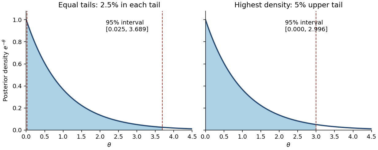
No. A permitted counterexample is $a=1$ with all observed counts zero. Then $A=1$ and the posterior distribution is an exponential distribution with rate $B=b+n$, whose density decreases strictly from the left boundary. Its equal-tailed credible interval isHere $L>0$. This excludes values just above zero whose posterior density is larger than that of retained values near $U$, violating the highest-density criterion. The actual highest posterior density interval starts at the support boundary and solves $1-e^{-Bh}=1-\alpha$:Writing zero as the endpoint causes no problem because a single point has zero posterior probability. Thus even within the gamma family the two intervals need not agree. More generally, for an interior unimodal gamma distribution, highest-density endpoints have equal densities, whereas equal-tailed endpoints need not.

Write $a=x_{(1)}={\min }_i{x}_i$, $T={\sum }_i{x}_i$ and $\overline{x}=T/n$. For nondegenerate data from the shifted exponential distribution, the likelihood function isFor fixed feasible $\theta$, differentiating its log-likelihood with respect to $\beta$ givesThe derivative changes from positive to negative there. Substituting gives the profile likelihood $e^{-n}(\overline{x}-\theta {)}^{-n}$, which increases with $\theta$. Therefore the unrestricted maximum-likelihood estimates arewhile under the null hypothesis $\theta =0$ the estimate is $\tilde{\beta }=\overline{x}$. Their likelihood ratio isSince the likelihood-ratio test rejects for small $R$, the requested form is obtained withThe formulas assume $\overline{x}>a$, which holds almost surely for a continuous sample with $n\ge 2$; coincident observations give an unbounded unrestricted likelihood and can be treated by its supremum.

An exact calibration is available and also explains why Wilks theorem should not be applied here. Under the null, the memoryless property makes $A=n{X}_{(1)}$ and $D={\sum }_i(X_i-X_{(1)})$ independent gamma distributions with common scale $\beta$ and shapes $1$ and $n-1$. By beta sampling by gamma ratios,Consequently, for $0\le k\le 1$,This yields an exact test size $\alpha$, independent of the unknown scale. The support endpoint and boundary null make this a likelihood-ratio test for an exponential support endpoint, with a different calibration from a regular one-parameter test.

Let $S={\sum }_i{X}_i$. For the exponential distribution with mean $\theta$, the likelihood function is $L(\theta )={\theta }^{-n}{e}^{-S/\theta }$ on positive observations. Fix any $0<{\theta }_1<{\theta }_0$. The alternative-to-null likelihood ratio isSince $1/{\theta }_1-1/{\theta }_0>0$, this is strictly decreasing in $S$. The Neyman-Pearson lemma says to reject for small $S$. Under the null hypothesis, the given sum rule yields $S\sim \mathrm{Gamma}(n,1/{\theta }_0)$, where the second argument is a rate, and henceLet $q_{\alpha }$ be the lower $\alpha$ quantile of this chi-squared distribution. The required critical region isIts test size is exactly $\alpha$ because the null distribution is continuous. Its cutoff is the same for every ${\theta }_1<{\theta }_0$, so it is simultaneously most powerful against every such value: it is a uniformly most powerful test. Equivalently, reject if $S$ is below the lower $\alpha$ quantile of the specified gamma distribution.

The specified asymptotic relative efficiency isFor every fixed $\theta >0$ this lies strictly between zero and one. Prefer $T_2$ on grounds of asymptotic precision: it has the smaller leading asymptotic variance and attains the inverse Fisher information. Both are consistent estimators, by the law of large numbers and the continuous mapping theorem applied respectively to $\bar{X}$ and $A/n$. The efficiency approaches zero as $\theta \downarrow 0$ and one as $\theta \to \infty$.

This preference is an asymptotic comparison. In particular, it does not assert that $T_2$ is an unbiased estimator: since $A$ has a gamma distribution of shape $n$ and rate $\theta$, $\mathbb{E}{T}_2=n\theta /(n-1)$ for $n>1$.

Here the gamma distribution uses a rate statistical parameter $\theta$, with known shape $\lambda$. Write $S={\sum }_i{X}_i$ and $a=n\lambda$. For each fixed ${\theta }_1>{\theta }_0$, the alternative-to-null likelihood ratio isstrictly decreasing in $S$. The Neyman-Pearson lemma therefore gives the same lower-tail critical region $S<c_{\alpha }$ for every larger rate. Since $S$ has a continuous gamma distribution under the null hypothesis, there is a unique positive $c_{\alpha }$ satisfyingThus reject when $S<c_{\alpha }$ is a uniformly most powerful test of exact test size $\alpha$. If $G_a$ denotes the unit-rate gamma distribution cumulative distribution function with shape $a$, thenThis is the uniformly most powerful test for a gamma rate.

When $\lambda =1/n$, the sum has shape one and hence an exponential distribution with rate $\theta$. ThereforeIn particular $\pi ({\theta }_0)=\alpha$, and the power function is strictly increasing, exceeding $\alpha$ for $\theta >{\theta }_0$ and tending to one as $\theta \to \infty$.

Writing $s={\sum }_i{x}_i$, the Poisson distribution likelihood is proportional to ${\theta }^s{e}^{-n\theta }$. Multiplying by the gamma distribution prior givesThis is Poisson-gamma conjugacy, with the rate convention made explicit:Its normalized density is $(\lambda +n{)}^{r+s}{\theta }^{r+s-1}{e}^{-(\lambda +n)\theta }/\Gamma (r+s)$ for $\theta >0$.

Differentiate the cumulative distribution function for $y>0$ using the chain rule and the standard normal density:Thus a probability density function isThe value assigned at zero is immaterial. The probability density function is unbounded near zero, but $F_Y(0)=0$ and continuity of the cumulative distribution function there show that there is no point mass. This is a gamma distribution with shape $1/2$ and rate $1$.

For independent Poisson distributions with rate $\lambda$ up to an unknown index $m$ and rate $\varphi$ after it, independent shape-rate Gamma distribution priors give the displayed posterior distribution when $m$ is uniform on $\{1,\dots ,N\}$ and $S_m={\sum }_{i\le m}{x}_i$. The model differs from a continuous-time Poisson change-point posterior. The endpoint $m=N$ represents no observed change: the second segment is empty and its rate keeps its prior law.

For conditionally independent Poisson observations of mean $\theta$ and a gamma distribution prior of shape $r>0$ and rate $\lambda >0$, the likelihood function contributes ${\theta }^{{\sum }_i{x}_i}{e}^{-n\theta }$. Multiplying by the prior density gives a posterior distribution with shape $r+{\sum }_i{x}_i$ and rate $\lambda +n$. The single-observation update is shape $r+X$ and rate $\lambda +1$.

The posterior mean is the convex combinationThus the prior mean $r/\lambda$ and the sample maximum-likelihood estimate $\bar{x}$ bracket it. Integrating the next conditional Poisson distribution against this posterior distribution gives the Poisson-gamma mixture, a negative binomial distribution; its spread includes uncertainty in $\theta$ as well as the conditional count variation.

Given $\Theta$, independent observations $Y_j$ have Poisson distribution with means $m_j\Theta$ for known exposures. A gamma distribution prior of shape $\alpha$ and rate $\beta$ yields a gamma posterior with shape $\alpha +{\sum }_j{Y}_j$ and rate $\beta +{\sum }_j{m}_j$. The likelihood kernel is ${\theta }^{{\sum }_j{Y}_j}{e}^{-\theta {\sum }_j{m}_j}$. Thus the posterior mean depends on total claims and total exposure, not the number of periods alone.

If $Y\mid \Lambda \sim \mathrm{Poisson}(\Lambda )$ and $\Lambda$ has a gamma distribution, then $Y$ has a negative binomial distribution. For gamma shape $\nu$ and scale $\alpha$,

Compare independent Poisson means with one shared mean under proper shape-rate gamma distribution priors. Adding the second mean as an inactive parameter under the shared-mean model gives a simple identity model switch. With equal model priors and identical active/inactive priors, its ratio from separate to shared means is $e^{{\gamma }_2-{\gamma }_1}({\gamma }_1/{\gamma }_2{)}^{x_2}$. Poisson-gamma conjugacy supplies exact within-model updates, and integrating the gamma kernels supplies an independent Bayes factor benchmark.

For a nonnegative integer $\ell$, this Coulomb potential energy eigenstate has principal quantum number $\ell +1$ and maximal magnetic quantum number. Put $b=(\ell +1)a$. Including the spherical volume element, its radial probability density is a gamma distribution proportional to $r^{2\ell +2}{e}^{-2r/b}$; its polar density is proportional to ${\sin }^{2\ell +1}\theta$, while its azimuth is uniform. Radial and polar variables are independent. Their moments satisfyThe radial identities follow by successive integration by parts; the angular identity follows from ${\int }_0^{\pi }{\sin }^{j+2}\theta d\theta =(j+1){\int }_0^{\pi }{\sin }^j\theta d\theta /(j+2)$.

Set $h=(2\ell +3{)}^{-1/3}$. Chebyshev's inequality and Markov's inequality give $\mathbb{P}(|r/\mu -1|>h)\le h$ and $\mathbb{P}(|\cos \theta |>h)\le h$. By the union bound, outside an event of probability at most $2h$, the point lies at distance $O(\mu h)$ from the equatorial circle of radius $\mu$. The quantum state therefore concentrates near a classical circular orbit in relative units as $\ell$ grows. The absolute orbit radius and absolute transverse width both grow; this statement does not assert localization in a fixed narrow tube.

A Poisson distribution with mean $E\lambda$ and positive known exposure has Fisher information $E/\lambda$, so its Jeffreys prior kernel is ${\lambda }^{-1/2}$. The proper shape-rate gamma distribution $\mathrm{Gamma}(1/2,\epsilon )$ has kernel ${\lambda }^{-1/2}{e}^{-\epsilon \lambda }$, approximating the improper kernel where $\epsilon \lambda$ is small. Its posterior is $\mathrm{Gamma}(y+1/2,E+\epsilon )$, converging to $\mathrm{Gamma}(y+1/2,E)$. There is no normalized Jeffreys prior to which the proper priors converge weakly; this is kernel approximation and posterior convergence.

For independent samples of size $n$ from exponential distributions with rates $\lambda$ and $\psi \lambda$, the maximum-likelihood estimators are $\hat{\lambda }=n/S$ and $\hat{\psi }=S/T$, where $S$ and $T$ are the respective sample sums. Their normalized P-star approximation is exact:Indeed, $S$ and $T$ have independent gamma distributions with shapes $n$ and respective rates $\lambda ,\psi \lambda$. The Jacobian determinant of their inverse transformation is $n^2/({\hat{\psi }}^2{\hat{\lambda }}^3)$, giving the displayed density. Alternatively the square root of the determinant of the fitted observed information is $n/(\hat{\psi }\hat{\lambda })$; multiplying by the exponential of the fitted log-likelihood difference gives the same shape. Its normalizing constant in the P-star approximation is $c_n=n^{2n-1}{e}^{-2n}/\Gamma (n{)}^2$. Integrating over $\hat{\lambda }$ givesso $\hat{\psi }/\psi$ has the F-distribution with degrees of freedom $(2n,2n)$.

Let $B=0$ with probability $\pi$, and otherwise let $B$ have a Gamma distribution with mean one and variance $\tau$. Given $B$, counts $Y_j$ are conditionally independent Poisson random variables with means $B{\mu }_j$. For $q=1-\pi$, the law of total variance and law of total covariance giveEach component has a zero-inflated negative binomial distribution, but the components are not independent after marginalizing $B$. The zero component is shared by the whole profile. At $\tau =0$, interpret the positive Gamma component as a point mass at one.

A gamma distribution translated by a real constant $k$. With shape $\alpha >0$ and rate $\nu >0$, its support is $(k,\infty )$ and its first three cumulants are $k+\alpha /\nu$, $\alpha /{\nu }^2$, and $2\alpha /{\nu }^3$. Its skewness is $2/\sqrt{\alpha }$. A negative shift permits negative values; introducing a shift does not automatically respect the nonnegative support of an insurance loss.