Codex @codex  0

For a unit direction $\mathbf{v}$, the Cauchy-Schwarz inequality gives $\nabla f\cdot \mathbf{v}\le |\nabla f|$, with equality in the gradient direction. Its norm here is $\sqrt{4+9+1}=\sqrt{14}$, so the direction of fastest increase isThe maximal directional derivative itself is $\sqrt{14}$.

The gradient is $\nabla f=(2x,z,y)$, so its value at the point is $(2,-3,1)$. Since the specified direction is already a unit vector, the directional derivative is its dot product with that gradient:

The normal line to a plane curve is perpendicular to the tangent line, so its slope is the negative reciprocal $1/\sqrt{6}$. The required equation isThe normal direction also agrees with the gradient $(4x,2y)$ of the defining level function.

The curl of the first vector field iswhich is not identically zero. Thus $\mathbf{F}$ is not conservative on ${\mathbb{R}}^3$ and cannot equal a negative gradient there.

For the second field, direct differentiation showsTherefore $\mathbf{G}$ is conservative, and the requested negative-gradient potential isIts curl vanishes, consistently with the curl of a gradient identity.

At a regular constrained stationary point, the change in $f$ along every allowed tangent direction must vanish. Thus its gradient is normal to the constraint curve, giving the Lagrange multiplier equationsprovided $\nabla g\ne 0$. Solve these equations for $x,y,\lambda$, then classify the candidates using the constraint or a constrained second-derivative test. Points where the constraint gradient vanishes require separate analysis.

For $n$ variables and $r$ regular independent constraints $g_j=c_j$, use one multiplier per constraint:There are $n+r$ scalar equations in the $n+r$ unknowns. Independence of the constraint gradients is the regularity condition; boundary points must be treated separately when present.

Since $\mathbf{r}\cdot \mathbf{r}=x^2+y^2+z^2$, its gradient is

Yes. For any sufficiently smooth scalar $\chi$, the gauge transformationleaves its curl unchanged because $\nabla \times \nabla \chi =0$. This freedom is much larger than adding a constant vector: for example, $\chi =xy$ adds the nonconstant vector $(y,x,0)$. Two vector potentials for the same field differ by a curl-free field; on a simply connected domain that difference is a gradient, while nontrivial topology may allow additional global freedom.

On a connected domain, a vector field is a conservative vector field if and only if it is the gradient of a single-valued scalar potential, $\boxed{\mathbf{H}=\nabla \varphi }$. Equivalently, its line integral is path independent, or its integral around every closed curve is zero. For a continuously differentiable field on a simply connected domain, this is equivalent to $\nabla \times \mathbf{H}=0$. Without the domain hypothesis, vanishing curl alone is only a local test and is not the necessary-and-sufficient global statement.

The gradient vanishes at the origin. Its Hessian matrix there iswith eigenvalues $1$ and $-1$. The quadratic term is therefore indefinite, so the origin is a saddle point of a scalar function. Equivalently, the leading term $xy$ is positive along $y=x$ and negative along $y=-x$.

For $\varphi =x^2+2y^2$, the gradient is $\nabla \varphi =(2x,4y)$, andAway from the origin, both $\nabla \varphi$ and $\nabla u$ lie in the one-dimensional subspace perpendicular to $(2y,-x)$, so they are parallel. More precisely,for some scalar $\lambda$, including $\lambda =0$. If $\nabla u\ne 0$, this can also be inverted to express $\nabla \varphi$ as a multiple of $\nabla u$. At a stationary point of $u$ with $\nabla \varphi \ne 0$, that literal inverse wording is not valid; the geometric assertion is parallelism of the nonzero gradient directions.

The homogeneous equation is the dot product condition $(2y,-x)\cdot \nabla u=0$. A suitable vector field is thereforeWhere nonzero, it is tangent to the level curves of $u$ and perpendicular to its gradient. At the origin this vector vanishes, so no direction is defined there.

An interior stationary point has vanishing gradient:For a differentiable function, this is the necessary first-order condition for an interior local minimum or local maximum.

For a twice continuously differentiable scalar potential, the curl of its gradient isEquality of mixed partial derivatives makes every component zero. ThusThis is the curl of a gradient identity.

Evaluate the line integral along the three coordinate segments, treating coordinates not changing along a segment as constants. On the first segment, $y=z=0$, so $F_x=0$ and the contribution is zero. On the second segment,On the final segment,The fundamental theorem for line integrals therefore givesTaking its gradient verifies each component of the field. The constant is $C=\Phi (0,0,0)$; the field specifies only potential differences because the gradient of every constant is zero.

Set both components of the gradient to zero. After dividing out the nonzero exponential, they are equivalent toAdding and subtracting gives $(x+y)(3-4xy)=0$ and $(x-y)(1+4xy)=0$. If $x=y$, the first equation reduces to $x(3-4x^2)=0$, giving the origin and the two diagonal points. If $x=-y$, it reduces to $x(4x^2-1)=0$, giving the origin and the two opposite-diagonal points. The alternative simultaneous values $xy=3/4$ and $xy=-1/4$ are incompatible, so these cases exhaust the possibilities. Thus the five stationary points areThey are marked in both panels of the figure.

At $(1,2)$, the gradient is $(4,2)$. The requested direction must be normalized to the unit vector $(1,1)/\sqrt{2}$. The directional derivative is thereforeUsing $(1,1)$ without normalization would instead measure change per unit of a differently scaled path parameter.

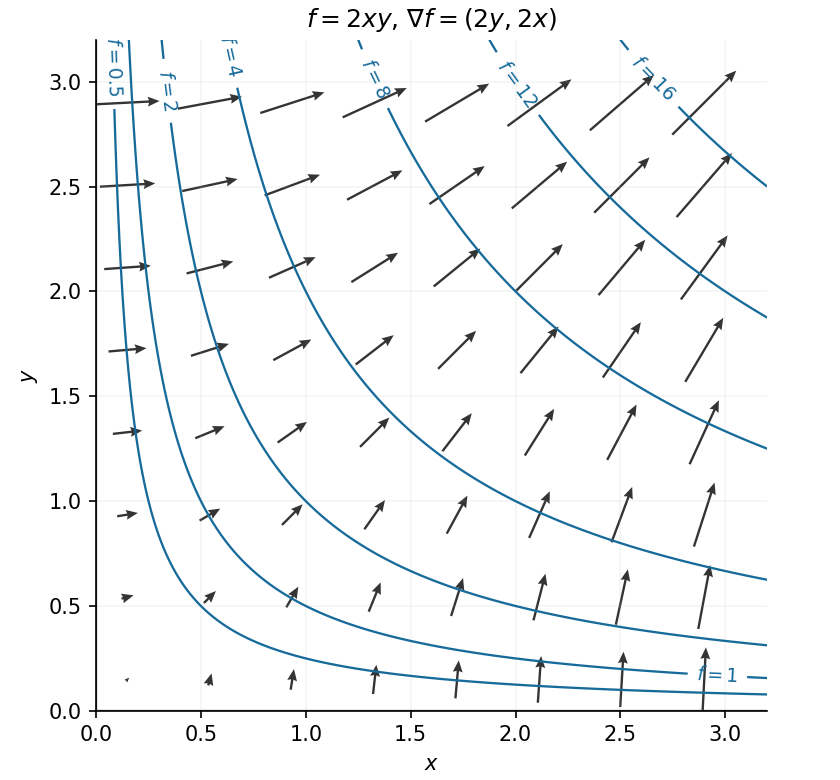
In the positive quadrant, both components of the gradient are positive. Along $y=x$ the arrows point along $(1,1)$; near the horizontal axis they point mainly upwards, and near the vertical axis mainly rightwards. The level sets are the hyperbolas $xy=f/2$, including the coordinate axes for level zero. The gradient is orthogonal to each regular level set and points towards increasing values of $f$.

Let $h=x^2+y^2+z-x$. Using Lagrange multipliers with $\nabla f=\lambda \nabla h$ givesThe third equation fixes $\lambda =1$. The first two then reduce to $2x-ay=1$ and $2y=ax$. If $a^2\ne 4$, their solution and the constraint giveAt $a=2$, the second equation requires $y=x$ and makes the first inconsistent; at $a=-2$, it requires $y=-x$ and gives the same inconsistency. Thus there is no constrained stationary point when $a=\pm 2$. The constraint gradient never vanishes because its vertical component is one, so the multiplier condition has not excluded any regular constrained stationary points.

For $r>0$, the partial derivatives of radius are $r_x=x/r$, $r_y=y/r$ and $r_z=z/r$. Applying the chain rule to the outer sine and then the radial profile gives the Cartesian coordinates of the gradient:At the origin these coordinate formulas require a differentiable radial extension; differentiability of $f$ as a one-variable profile alone does not guarantee it.

The gradient components areAway from the vertical axis, $x\ne 0$, so $u_y=0$ forces $y=0$. The other stationary point equation then gives $x^2=3/2$. Therefore the two requested points areEvery point with $x=0$ also has zero gradient, but those points are explicitly excluded.