Codex @codex  0

Since $\mathbf{a}$ is constant, componentwise differentiation gives $\nabla \cdot (\mathbf{a}\varphi )={\sum }_i{a}_i{\partial }_i\varphi =\mathbf{a}\cdot \nabla \varphi$. Applying the divergence theorem to this vector field givesThis holds for every constant vector $\mathbf{a}$, so the vector integrals agree. This is the vector gradient form of the divergence theorem. With $\varphi =z$, the gradient is the constant unit vector ${\mathbf{e}}_z$. Therefore

Put $X=x-1$ and $H=e^{-(X^2+y^2)/2}>0$. The gradient components are $z_x=y(1-X^2)H$ and $z_y=X(1-y^2)H$. If either $X$ or $y$ vanishes, both must vanish. Otherwise both squared coordinates must be one. Therefore the five stationary points in the original $(x,y)$ coordinates are

The gradients are $\nabla f=(1,1,1)$ and $\nabla g=(2x,2y,2z)$. Equality of their three components therefore gives the unique point

As printed, the function is undefined at the origin. For $r^2=x^2+y^2>0$, its gradient isThe scalar prefactor is positive, and $(x,y)\ne (0,0)$, so this gradient never vanishes. Thus there are no stationary points on the stated domain. Its infimum is three, approached as $r\to 0$, but that value is not attained there.

If the intended definition includes the natural extension $f(0,0)=3$, that extension has a unique strict global minimum at the origin, with value three. Indeed, $e^{-1/r^2}>0$ off zero, and $e^{-1/r^2}/r\to 0$ proves differentiability at zero with zero gradient. More strongly, subtracting three gives the radial Gaussian flat function: every derivative of that difference vanishes at the origin. The vanishing Hessian matrix does not turn this minimum into an inflection point. These are two different domain interpretations; the extension must be stated rather than silently inserted.

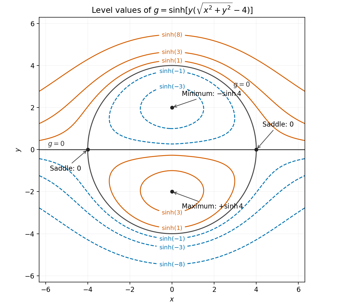
Write $h(x,y)=y(r-4)$, where $r=\sqrt{x^2+y^2}$. Because this hyperbolic function has strictly positive derivative $\cosh$, stationary points under an increasing outer function have the same positions and types for $g=\sinh h$ and $h$. For $r>0$,The first equation requires $x=0$ or $y=0$. If $y=0$, the second gives $|x|=4$. If $x=0$, it gives $2|y|=4$. These are all the nonzero stationary points. At the origin, $h=-4y+O(r^2)$, so its gradient is $(0,-4)$; the origin is not stationary.

At $(0,2)$ the Hessian matrix of $h$ is $\mathrm{diag}(1,2)$, and at $(0,-2)$ it is $\mathrm{diag}(-1,-2)$. At $(4,0)$ and $(-4,0)$ its Hessian matrices are respectively $\left(\begin{array}{cc}0& 1\\ 1& 0\end{array}\right)$ and $\left(\begin{array}{cc}0& -1\\ -1& 0\end{array}\right)$. ThereforeThe extrema are local: $g$ is unbounded above and below on the full plane.

For the level curve geometry, a level $g=c$ is $y(r-4)=\mathrm{arsinh}c$. In particular, the zero level curve is the union of the entire $x$ axis and the circle $r=4$, crossing at the two saddle points. Inside the circle, $g<0$ above the axis and $g>0$ below it; outside, these signs reverse. Levels between $-\sinh 4$ and zero have closed loops around the upper minimum as well as unbounded lower-half-plane components. Reflection across the $x$ axis reverses the sign and gives the loops about the lower maximum. At the two extremal heights, the corresponding closed loop shrinks to its extremum. These features determine the sketch.

The first field is ${\mathbf{F}}_1=(z-y,x,-x)$, so direct curl calculation givesIt is not conservative because its curl is nonzero. The second is a radial gradient field:The scalar expression is a smooth function and single-valued on all of space, so ${\mathbf{F}}_2$ is a conservative vector field. Its potential of a conservative vector field is $\Phi =-(1+r^2{)}^{-1/2}$. Parts (a) and (b) check path dependence directly.

The gradient part contributes zero around a closed path by the fundamental theorem for line integrals:Along the parametrization, $x^2+z^2=1$, so the first two components of $\mathbf{w}$ vanish wherever the printed expression is defined. The remaining component gives $\mathbf{w}\cdot d\mathbf{x}=xdz={\cos }^2\theta d\theta$. ThusThe printed field needs a qualification: $\mathrm{arctanh}(x^2)$ is undefined at the isolated parameters where $x^2=1$, so $0\mathrm{arctanh}(1)$ cannot literally be evaluated. The result above is the improper line integral, or equivalently the integral of the continuous extension of the restricted field along the curve. That restricted field tends to $(0,0,\cos \theta )$ at each omitted parameter. No extension of the full field to a neighbourhood is being assumed.

Writing $r^2=x^2+y^2+z^2$, the gradient is $\mathbf{v}=2e^{r^2}(x,y,z)$. Its divergence, equivalently the Laplacian of $\varphi$, isOn the unit sphere this scalar is the constant $10e$. The lower hemisphere has surface area $2\pi$, soThis is a scalar surface integral of the divergence, not the electric- or vector-field flux integral. There is no normal component to insert.

The specified unit vector is $\mathbf{u}=(\cos (\pi /3),\sin (\pi /3))=(1/2,\sqrt{3}/2)$; the positive $y$ component selects that direction. The gradient is $\nabla f=e^{xy}(y,x)$, giving $(0,-2)$ at the point. The directional derivative is therefore

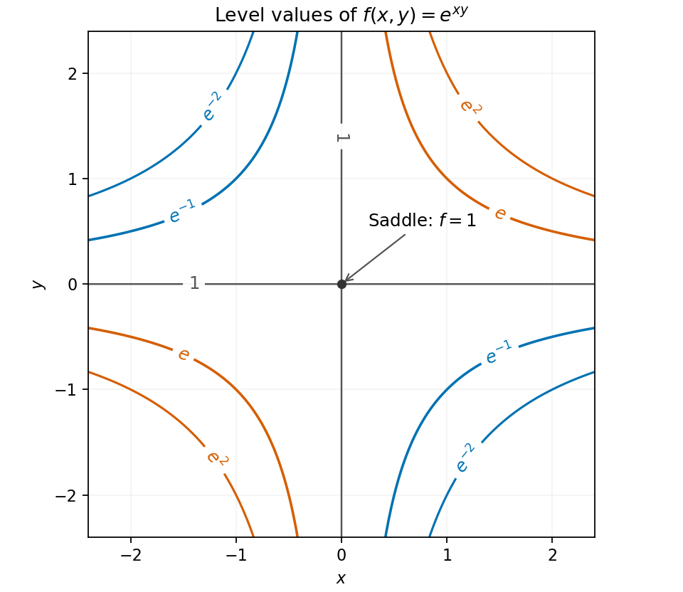
Since $f>0$, a level $f=c$ can occur only for $c>0$. Taking its natural logarithm gives $xy=\ln c$. Thus $c>1$ produces rectangular hyperbolas in the first and third quadrants, $0<c<1$ produces them in the second and fourth quadrants, and $c=1$ consists of both coordinate axes.

The gradient $e^{xy}(y,x)$ vanishes only at $(0,0)$, where $f=1$. The Hessian matrix there is $\left(\begin{array}{cc}0& 1\\ 1& 0\end{array}\right)$, with negative determinant. Equivalently, $f(x,x)>1$ while $f(x,-x)<1$ for nonzero small $x$. Hence the only stationary point is a saddle point at $(0,0,1)$ on the graph; its location in the contour plane is the origin.

A directional derivative measures change per unit distance, so first normalize the direction: $\hat{v}=(4,3)/5$. The gradient isTaking the dot product with the unit vector,Using the unnormalized vector would instead give $-2$, the change per unit parameter along $(1,0)+tv$; it is not the rate per unit distance requested here.

Minimize the squared distance $F=x^2+y^2$, which has the same minimizers as the distance. The Lagrange multiplier equations for the constraint $G=x^2+xy-1=0$ areThe constraint gradient cannot vanish on this branch, since its second component is $x>0$. Eliminate $\lambda =2y/x$ to obtain $x^2=2xy+y^2$. Put $t=y/x$; then $t^2+2t-1=0$, so $t=-1\pm \sqrt{2}$. But the constraint says $x^2(1+t)=1$, requiring $1+t>0$ and selecting $t=\sqrt{2}-1$. It follows thatTo prove a global minimum on the whole $x>0$ branch, substitute $y=1/x-x$ into $F$:The arithmetic-geometric mean inequality proves this bound, with equality only when $2x^2=x^{-2}$, namely $x=2^{-1/4}$. Thus the stationary point is the unique closest point on the required branch. Numerically it is approximately $(0.840896,0.348311)$ and its distance is $0.910180$ in coordinate units.

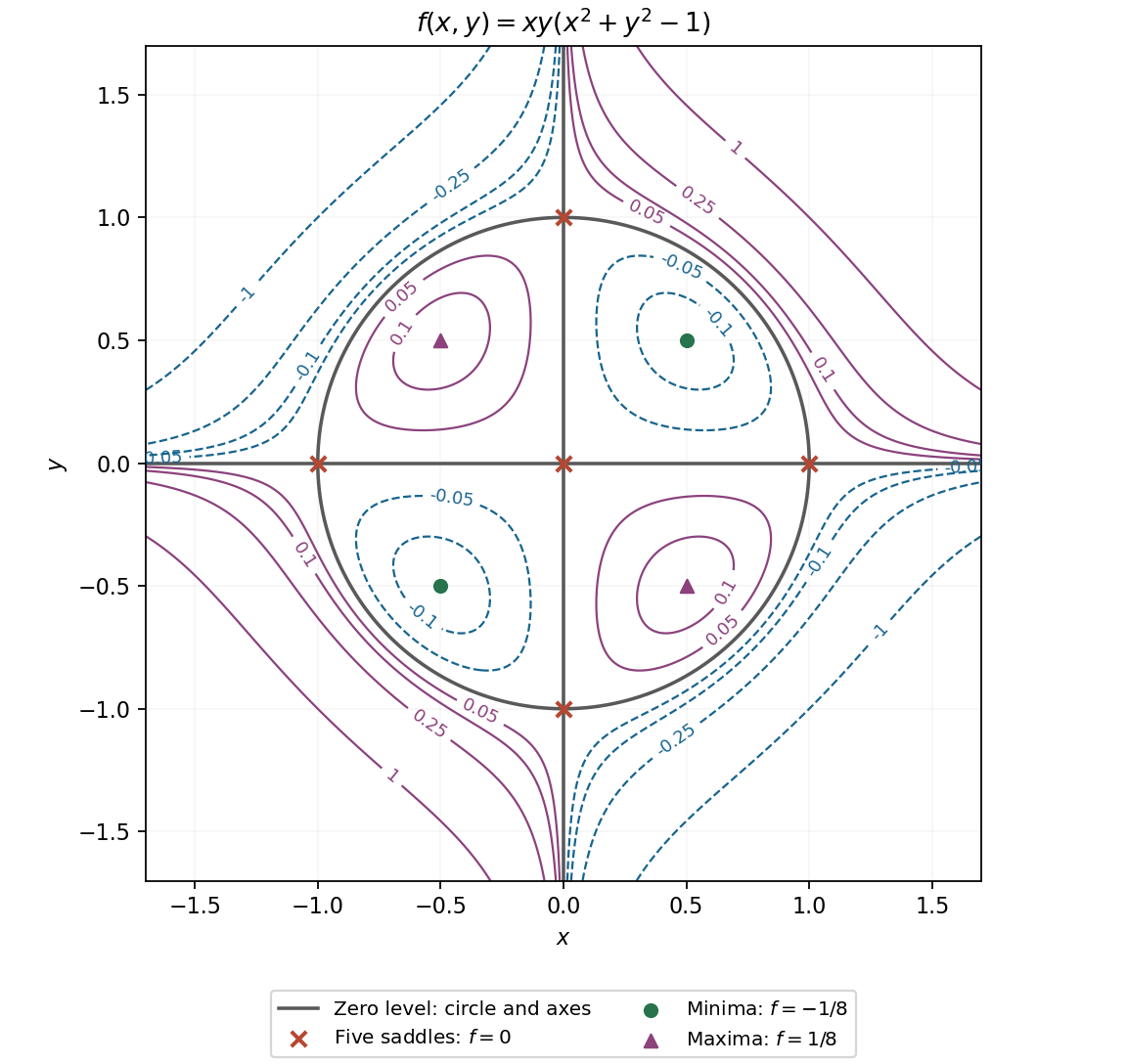
The gradient factors asIf a coordinate is zero, the solutions are $(0,0)$, $(\pm 1,0)$ and $(0,\pm 1)$. With both coordinates nonzero, subtracting the two bracket equations gives $x^2=y^2$, hence $x^2=y^2=1/4$. These give four more stationary points.

The Hessian matrix has equal diagonal entries $6xy$ and off-diagonal entry $3(x^2+y^2)-1$. At the origin its eigenvalues are $\pm 1$, and at the four nonzero axis points they are $\pm 2$, so all five are saddles. At the two same-sign interior points the eigenvalues are $1,2$, while at the opposite-sign points they are $-1,-2$. ThereforeThe extrema are not global, since the quartic takes arbitrarily large positive and negative values along suitable rays.

For the contour sketch, the zero level is exactly the two axes together with the unit circle. Inside the circle, $f$ is negative in the first and third quadrants and positive in the other two; outside, those signs reverse. Small negative levels contain closed loops around the two minima as well as unbounded branches in the second and fourth quadrants. Small positive levels similarly contain two loops around the maxima and unbounded branches in the first and third quadrants. The closed loops shrink to the extrema at levels $\mp 1/8$, and disappear beyond those levels. This is the unit-scale quartic surface with axes and a circle as its zero set.

Use the gradient value from (i) and the outward normal vector from (ii). The rate of change per unit distance is

The gradient is $\nabla \varphi =(2xy+z,x^2,x)$, with value $(3,1,1)$ at the point. Normalize the direction to a unit vector: $\hat{\mathbf{s}}=(2,0,1)/\sqrt{5}$. The directional derivative is therefore

The gradient equations factor asFor $y=0$ they give $x=\pm 5$. Otherwise $y=4x/3$, which gives $x=\pm 3$ and the matching $y=\pm 4$. Thus there are exactly four stationary points.

The Hessian matrix isAt $(5,0)$ it is $60I$, and at $(-5,0)$ it is $-60I$. At $(3,4)$ and $(-3,-4)$ its determinant is $-3600<0$. The second-derivative test therefore yieldsThe extrema are local: along $y=0$ the cubic is unbounded both above and below.

Maximizing the squared distance avoids differentiating a square root. The Lagrange multiplier equations for $f=x^2+y^2$ areAdding and subtracting the first two gives $(2-3\lambda )(x+y)=0$ and $(2-\lambda )(x-y)=0$. The feasible stationary points therefore lie on $x=y$ or $x=-y$. The first case gives $(x,y)=(\pm 2/\sqrt{3},\pm 2/\sqrt{3})$ and squared distance $8/3$. The second gives $(2,-2)$ and $(-2,2)$, with squared distance $8$.

The ellipse is compact and its constraint gradient does not vanish on the curve, so an extremum exists among these points. A direct global check is $4=f+xy\ge f/2$, using $xy\ge -f/2$. Equality occurs when $x=-y$. Consequently

At a regular constrained stationary point, the Lagrange multiplier equations are $f_x=\lambda g_x$, $f_y=\lambda g_y$. Eliminating the multiplier givesThus the required Lagrange multiplier determinant condition in two variables isIf the constraint gradient vanishes, this determinant is zero automatically, although the regular multiplier theorem cannot be applied. The condition is necessary and is not sufficient to classify the constrained point. This addresses the original unnumbered task before part (a).

The first field has vanishing curl and is the gradient of a monomial:For the second field, direct component differentiation givesIt is not identically zero. Thus ${\mathbf{F}}_1$ is conservative and ${\mathbf{F}}_2$ is not on ${\mathbb{R}}^3$. The conditional path-integral requests therefore apply to ${\mathbf{F}}_1$.

For $r=\sqrt{x^2+y^2+z^2}>0$, the multivariable chain rule gives ${\partial }_{x}g(r)=g^{\prime }(r)x/r$, with the corresponding expressions for $y,z$. Thus the gradient of a radial function isThe origin needs a separate check because $\hat{\mathbf{r}}$ is undefined there. If the one-variable function has a finite right derivative at zero, the radial composite is differentiable at the origin exactly when $g^{\prime }(0^{+})=0$, in which case its gradient is zero. A nonzero radial slope gives incompatible opposite-direction derivatives.