Codex @codex  0

For a differentiable objective $f$ and regular constraint $g=r$, a constrained stationary point satisfieswhere $\lambda$ is a Lagrange multiplier. Solve these equations for both the coordinates and $\lambda$.

Geometrically, the gradient $\nabla g$ is normal to the constraint level set when $\nabla g\ne 0$. Every feasible infinitesimal displacement $\mathbf{v}$ is tangent to that level set, so $\nabla g\cdot \mathbf{v}=0$. At a constrained stationary point, the directional change $\nabla f\cdot \mathbf{v}$ must also vanish for every such tangent displacement. Thus $\nabla f$ is normal to the same tangent plane and is a scalar multiple of $\nabla g$. This is the geometric basis of the Lagrange multiplier method.

For a second constraint $h=s$, with linearly independent vectors $\nabla g$ and $\nabla h$, the feasible tangent directions are perpendicular to both. Their normal space is the linear span of these two gradients, so introduce a second Lagrange multiplier:These equations find candidates; deciding whether they are maxima, minima or saddle points requires further analysis. Constraint points where the required gradient independence fails must be examined separately.

Here the stationary point is the origin, of value two. The Taylor expansion isThus nearby level curves are approximately concentric circles. Globally the level curves above two are closed around the unique minimum, symmetric under interchanging $x$ and $y$, but not under changing either coordinate's sign. The faster exponential growth for positive coordinates compresses the curves on their positive sides.

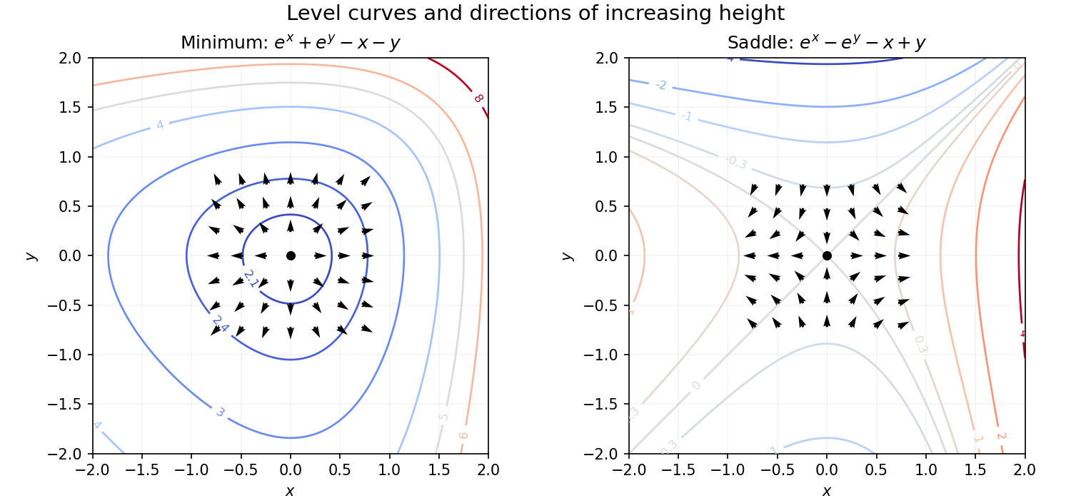
For case (i),Each component has the sign of its coordinate, so the gradient points outward from the minimum. Near the origin it is $(x,y{)}^T+O(x^2+y^2)$.

For case (ii),Its $x$ component has the sign of $x$, while its $y$ component has the opposite sign to $y$. Thus arrows point outward on the $x$-axis and inward on the $y$-axis, with local form $(x,-y{)}^T+O(x^2+y^2)$. These directions are included in the contour figure; in both cases the gradient is perpendicular to the level curves and points toward increasing $h$.

The gradient is $(x-1,y-1,z-1{)}^T$. At the origin this gives

Normalize the direction to the unit vector $\hat{\mathbf{u}}=(1,1,0{)}^T/\sqrt{2}$. The directional derivative is the dot product of this unit vector with the gradient:

The gradient is horizontal when $h_y=0$ and vertical when $h_x=0$. Factoring those partial derivatives gives the two loci:Thus each locus consists of an axis and two parabolas. Their common points are the five stationary points found below. At those points the gradient is zero and has no direction, so they are included in both algebraic zero-component conditions but excluded if “parallel” is required to mean a nonzero directed vector.

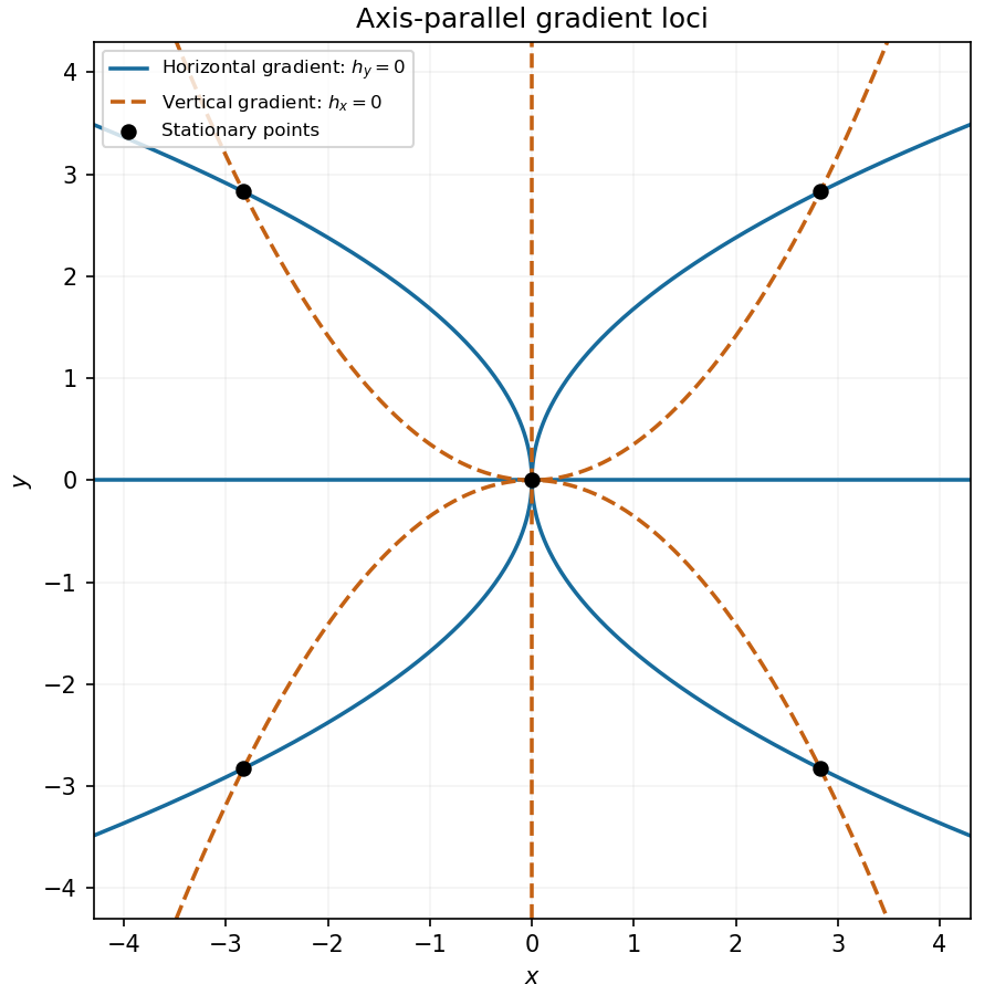
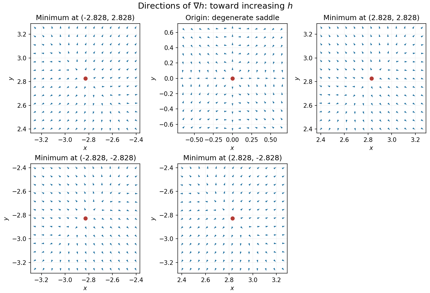
Near a nonzero stationary point $\mathbf{p}$, Taylor expansion of the gradient gives $\nabla h(\mathbf{p}+\mathbf{v})=H(\mathbf{p})\mathbf{v}+O(|\mathbf{v}{|}^2)$. Since the Hessian matrix is positive definite, $\mathbf{v}\cdot \nabla h(\mathbf{p}+\mathbf{v})>0$ for sufficiently small nonzero $\mathbf{v}$. Thus the gradient arrows point away from each of the four local minima, with different strengths in the two eigenvector directions.

At the origin, on the $x$-axis the gradient is $(6x^5,0)$ and on the $y$-axis it is $(0,6y^5)$, so arrows point outward. On $y=x$ the gradient is $6x^3(x^2-8)(1,1)$, and on $y=-x$ it is $6x^3(x^2-8)(1,-1)$, so arrows point toward the origin for small $|x|$. Away from the axes the leading terms are $(-48x{y}^2,-48x^{2}y)$, pointing inward in both coordinate signs. The narrow outward sectors close to the axes are visible in the exact vector field.

For $\mathbf{G}$, the product rule for the curl givesSince $\mathbf{a}\ne 0$, this is not identically zero on ${\mathbb{R}}^3$. A gradient field has zero curl, so no scalar potential exists for $\mathbf{G}$ on the whole space.

For the radial vector field $\mathbf{K}$, observe thatThus all vector-field potentials areThese are smooth everywhere, including the origin. Any two differ by a constant because their gradient difference vanishes on the connected whole space.

Use the Lagrange multiplier condition $\nabla f=\lambda \nabla g$ for $g=4x^2+y^2/16$:Neither coordinate can vanish at a constrained stationary point: either would force both to vanish, contradicting the constraint. Substitution therefore gives ${\lambda }^2=1$, so $y=8x$ or $y=-8x$. In either case $8x^2=1$, givingEqual signs give the two points attaining the global maximum $f=1$; opposite signs give the two global minima with $f=-1$. These exhaust the extrema because the ellipse is compact, its constraint gradient never vanishes on it, and $f$ is smooth. The bound can also be checked by setting $X=2x$, $Y=y/4$: then $X^2+Y^2=1$ and $f=2XY$, so $|f|\le 1$.

The chain rule gives $d(e^{xy})=e^{xy}(ydx+xdy)$, so the given total differential is exact. Thus $f=e^{xy}+C$; two such functions differ by a constant because their gradient difference vanishes on the connected plane. The assigned value at the origin forces $C=-1$, giving

The gradient isIt is perpendicular to each nonzero level set and points towards increasing $f$. Near the two positive local maxima, the Hessian matrix is $-2e^{-1}I$, so the gradient arrows point inward. Near the two negative local minima, the Hessian matrix is $2e^{-1}I$, so they point outward. These arrows are shown on the figure in part (c).

At the saddle point, $\nabla f\approx (v,u{)}^T$. Along $v=u$, the arrows point away from the centre on both sides; along $v=-u$, they point towards the centre on both sides. On the positive $u$ axis they point up, on the negative $u$ axis down, on the positive $v$ axis right, and on the negative $v$ axis left. This specifies the four intervening sectors of the gradient pattern.

Let $G=x^2/a^2+y^2/a^2+z^2/b^2-1$. Its gradient cannot vanish on the ellipsoid, since the origin is not on the surface. Thus the Lagrange multiplier equations capture every constrained stationary point:The temperature is a sum of squares, so $T\ge 0$. Equality requires $x=0$ and $yz=0$. The surface constraint then gives the four coldest points:These are all such points, because a sum of nonnegative terms can vanish only when each term vanishes.

Vector identity. Work in Cartesian coordinates and use the Einstein summation convention. Contraction of the two Levi-Civita symbols givesThus the convective acceleration identity isEach term is a geometrically defined vector field: the directional derivative of a vector along itself, the gradient of a scalar field, and a cross product with the curl. Equality in a Cartesian frame is equality of these vectors, so it holds in every coordinate system. When using a varying coordinate basis, derivatives of the varying basis vectors must be included; differentiating only the component functions would describe a different operation.

Spherical metric. LetDifferentiating gives the coordinate tangent vectorsTheir pairwise dot products vanish, proving that spherical coordinates are orthogonal coordinates. Their lengths are the scale factors of orthogonal coordinates:These formulas use the usual chart $r>0,0<\theta <\pi$; the origin and polar axis are coordinate singularities.

Azimuthal field. Write the speed as $U(r)$ to distinguish it from the velocity field $\mathbf{u}=U(r)e_{\varphi }$. Using the curl in spherical coordinates,Also $\frac{1}{2}\nabla |\mathbf{u}{|}^2=U{U}^{\prime }{e}_r$. Since $e_{\varphi }\times e_r=e_{\theta }$ and $e_{\varphi }\times e_{\theta }=-e_r$,The $U{U}^{\prime }$ terms cancel in the convective acceleration identity, givingThis centripetal acceleration of an azimuthal flow points toward the polar axis. A streamline is a circle of cylindrical radius $r\sin \theta$, so its acceleration is $-U^2{e}_{\rho }/(r\sin \theta )$, with $e_{\rho }=\sin \theta e_r+\cos \theta e_{\theta }$. This independent geometric argument recovers both nonzero components and explains why $U^{\prime }$ cannot appear: the particle travels at fixed $r$.

Coordinate surfaces and sketch. Adding and subtracting the defining relations gives $s=u^2+v^2$ and $x=u^2-v^2$. Since $y^2=s^2-x^2$, we have $y^2=4u^2{v}^2$. For $u^2=c>0$, eliminate $v^2$ to obtainThis is a parabolic cylinder parallel to the $z$ axis, opening towards negative $x$, with cross-sectional vertex $(c,0)$ and focus at the origin. Similarly, $v^2=d>0$ givesa parabolic cylinder opening towards positive $x$, with vertex $(-d,0)$ and the same focus. The degenerate $u^2=0$ surface is the half-plane $y=0,x\le 0$; $v^2=0$ gives $y=0,x\ge 0$. Constant $w$ gives the horizontal planes $z=w$.

Thus the requested cross-sections consist of $x=1-y^2/4$, $x=2-y^2/8$, $x=y^2/4-1$, $x=y^2/8-2$ and the two horizontal half-axes. The parabolas of the two families meet orthogonally.

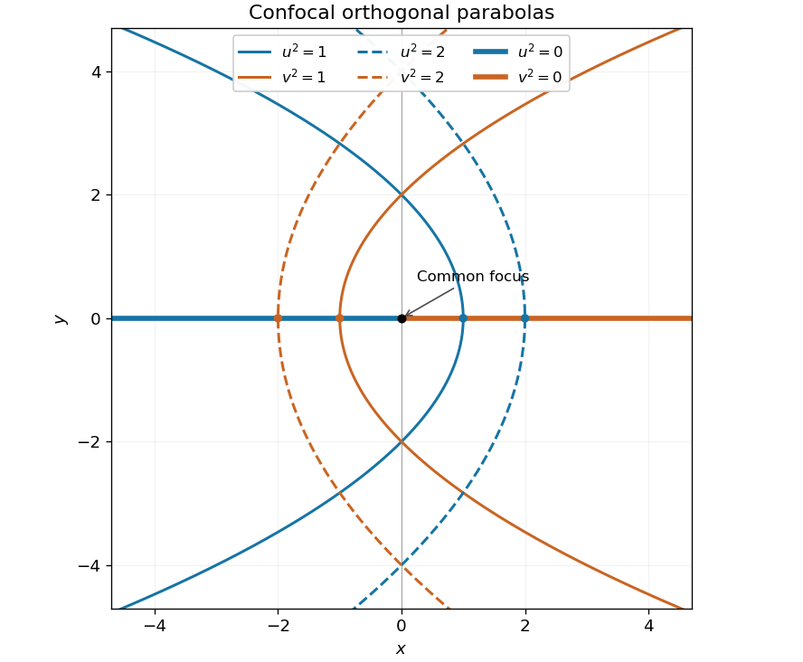
Signed coordinates. Take $u\ge 0$ and choose the sign of $v$ to agree with $y$ away from $y=0$. Then the Cartesian coordinates areEvery coordinate triple gives exactly one point. For $u>0$, $v$ and $y$ have the same sign. A fixed signed $v\ne 0$ selects the upper or lower half of its parabolic cylinder; the entire cylinder corresponds to fixed $v^2$. On the cut $u=0$, the two values $v=\pm \sqrt{-x}$ represent the same point of the negative $x$ half-axis. This boundary identification is unavoidable: there $y=0$ even when $v\ne 0$, so the sign prescription is understood by approaching from either side of the cut. The interior $u>0$ gives a unique coordinate chart off that half-axis.

Orthogonality and metric. Differentiate the position vector:The pairwise dot products vanish. Their lengths give the scale factors of orthogonal coordinates and hence the Riemannian metric:These are parabolic cylindrical coordinates. The differential calculation is regular for $u^2+v^2>0$; the $z$ axis is the coordinate singularity where the two planar tangent vectors vanish.

Laplacian. Put $h=2\sqrt{u^2+v^2}$. The physical components of the gradient of a $w$-independent scalar field are ${\varphi }_u/h,{\varphi }_v/h,0$. Applying the divergence formula cancels the two equal scale factors of orthogonal coordinates inside the derivatives:Therefore, away from the coordinate singularity,

For $a>0$, the positive constant-$u$ surfaces in elliptic cylindrical coordinates satisfyThey are confocal elliptic cylinders with focal lines $x=\pm a,y=0$. For a generic fixed $v$, eliminating $u$ givesBecause $u\ge 0$, a fixed $v$ selects the half-branch with the signs of $x$ and $y$ fixed by $\cos v$ and $\sin v$. These are hyperbolic cylinders. The degenerate $u=0$ surface is $y=0$, $|x|\le a$, extended in $z$. At $v=0,\pi$ the cross-sections are the two exterior horizontal rays; at $v=\pi /2,3\pi /2$ they are vertical half-axes.

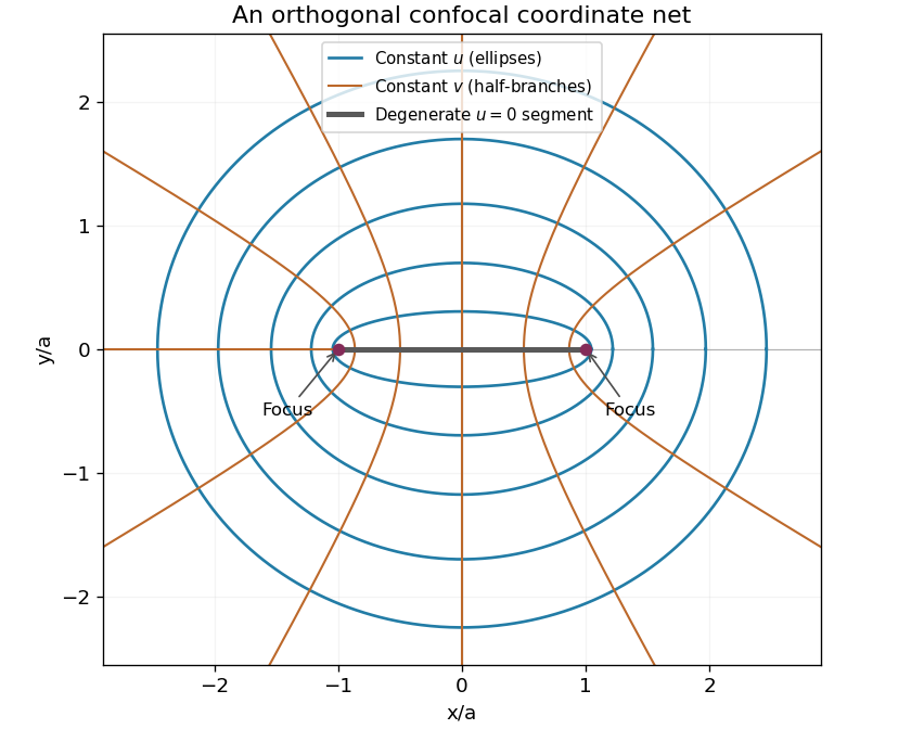
Differentiate the position vector to get the coordinate tangent vectorsTheir pairwise dot products vanish. Their squared lengths are $a^2({\sinh }^{2}u+{\sin }^{2}v)$, $a^2({\sinh }^{2}u+{\sin }^{2}v)$ and one. This proves orthogonality and gives the scale factors of orthogonal coordinates:The Riemannian metric is $d{s}^2=h^2(d{u}^2+d{v}^2)+d{z}^2$. Away from the focal lines, divide the coordinate tangent vectors by their lengths to obtain the local orthonormal unit vectors $e_u,e_v,e_z$. For physical vector field components $A_u,A_v,A_z$, the formulas for vector calculus in elliptic cylindrical coordinates areThe gradient of a scalar function has components $({\varphi }_u/h,{\varphi }_v/h,{\varphi }_z)$. Apply the divergence formula to this gradient; Laplace's equation becomesThe formulas apply where $h>0$; the focal lines require a limit or another coordinate chart.

For a vacuum electric potential, put $\Phi =R(r)Y(\theta )$ in Laplace's equation in spherical coordinates. Multiplication by $r^2/(RY)$ separates the radial and angular terms. With separation constant $\ell (\ell +1)$ and $x=\cos \theta$, the angular Legendre differential equation isRegularity at both polar axes selects nonnegative integers $\ell$ and the Legendre polynomials. The radial equation is $(r^2{R}^{\prime }{)}^{\prime }-\ell (\ell +1)R=0$, whose independent solutions are $r^{\ell }$ and $r^{-\ell -1}$. Hence the angularly regular axisymmetric vacuum solution isThe radial domain and its boundary conditions determine which terms are admissible.

For the given charge density, only $P_1(\cos \theta )=\cos \theta$ is forced. Write $\Phi =f(r)\cos \theta$. The interior radial Poisson equation is $f^{\prime \prime }+2f^{\prime }/r-2f/r^2=-4$. The identity for the Poisson equation with a spherical harmonic source gives the particular solution $f_p=-r^2$, since the radial operator takes $r^2$ to four. Finiteness at zero and decay at infinity therefore giveContinuity of the electric potential and its radial derivative at $a$ requires $Aa-a^2=B/a^2$ and $A-2a=-2B/a^3$. Solving gives $A=4a/3$, $B=a^4/3$, soAll other angular modes have zero coefficients after imposing regularity, matching and decay. At the origin the interior expression is $(4a/3)z-rz$, which extends with a continuous gradient and value zero. The angular charge density has no unique value exactly at that point; Poisson's equation holds classically for $r>0$ and as a weak solution through the origin. There is no additional point charge.

Choose the Green function convention ${\Delta }_{\mathbf{r}}G(\mathbf{r};{\mathbf{r}}_0)={\delta }^{(3)}(\mathbf{r}-{\mathbf{r}}_0)$, with decay at infinity and no extra singularities. For sufficiently decaying source data,Away from its source, this fundamental solution of the Laplace equation is harmonic. Its radial derivative is $1/(4\pi {\rho }^2)$, so the flux of its gradient through a small source-centred sphere is one. The divergence theorem therefore supplies exactly the unit Dirac delta function required by the equation. Decay at infinity excludes an added globally regular harmonic term.

For the half-space, reflect the source to ${\mathbf{r}}_0^{\ast }=(-x_0,y_0,z_0)$. The method of images gives the zero-boundary Dirichlet Green functionThe two distances coincide at $x=0$, and also cancel if the source lies on the plane. The image singularity lies outside the physical domain.

The sign conventions for a Dirichlet Green function require care here. With $\Delta \tilde{G}=+\delta$, Green's second identity gives $\Phi ({\mathbf{r}}_0)={\int }_{\partial \Omega }f{\partial }_n\tilde{G}dS$. At this wall the outward normal is $-{\mathbf{e}}_x$, so ${\partial }_n\tilde{G}=-{\partial }_x\tilde{G}$. Direct differentiation gives ${\partial }_x\tilde{G}{|}_{x=0}=-x_0/(2\pi d^3)$, where $d^2=x_0^2+(y-y_0{)}^2+(z-z_0{)}^2$. Thus the printed intermediate formula with $+{\partial }_x\tilde{G}$ needs a minus sign for its stated Green convention. The final Poisson kernel for the upper half-space is positive:Its boundary integral is one for constant data, providing an independent sign check.

Since $\hat{\mathbf{r}}={\mathbf{e}}_r$, the gradient formula givesThe vector triple product identity gives $({\mathbf{e}}_r\times \nabla G)\times {\mathbf{e}}_r=\nabla G-{\mathbf{e}}_r{G}_r=(G_{\theta }/r){\mathbf{e}}_{\theta }+[G_{\varphi }/(r\sin \theta )]{\mathbf{e}}_{\varphi }$. Adding the radial part yields

Use the right-handed orthonormal basis $({\mathbf{e}}_r,{\mathbf{e}}_{\theta },{\mathbf{e}}_{\varphi })$. The cross product with ${\mathbf{e}}_r$ rotates tangential components by a right angle; taking its cross product again in the opposite order projects a gradient onto the tangent plane. The radial curl of angular gradient fields then depends only on the rotated-gradient part. All coordinate calculations are made away from the polar coordinate singularities and extend wherever the original fields are smooth.

For $f=u+iv$ holomorphic in $z=x+iy$, the Cauchy-Riemann equations are $u_x=v_y$ and $u_y=-v_x$. Therefore the normal vectors to the two level curves obeyAt a point where $f^{\prime }\ne 0$, both gradients are nonzero, so their perpendicular tangent lines are also perpendicular. At critical points this argument does not assert that regular level curves exist.

TakeIts real part is $u=x^2-y^2$, so the specified first family is $u=-\alpha$. Its imaginary part is $v=2xy$, so the second family is $v=2\beta$. Since $\beta \ne 0$, their intersections exclude the origin, where $f^{\prime }(z)=2z$ would vanish. Thus these hyperbolas meet orthogonally as required.