Codex @codex  0

Put $d=1-x^{T}x>0$. Differentiating the barrier gradient givesAt a nonzero stationary point on the branch $Ax={\lambda }_{1}x$, $\mu /d=-{\lambda }_1$. Choose an orthonormal eigenbasis of the symmetric matrix $A$ whose first vector is $x/\Vert x{\Vert }_2$. On each of the remaining eigenvectors the rank-one term vanishes, so the corresponding Hessian eigenvalues areAlong $x$, the first two terms cancel and the remaining eigenvalue isIf ${\lambda }_1$ repeats, a transverse eigenvalue can be zero. If a lower eigenvalue than ${\lambda }_1$ exists, a transverse eigenvalue is negative, identifying this stationary branch as a saddle rather than a minimum.

A line search chooses a positive step size giving useful decrease along the chosen direction. Fix $\sigma ,\beta \in (0,1)$ and a trial step $\bar{\alpha }>0$. The Armijo condition isThe backtracking line search tests $\bar{\alpha },\beta \bar{\alpha },{\beta }^2\bar{\alpha },\dots$ and takes the first accepted value. A Lipschitz gradient has $\Vert \nabla f(y)-\nabla f(x){\Vert }_2\le L\Vert y-x{\Vert }_2$ with a constant $L$ independent of $x,y$.

Integrating the gradient along a segment gives the descent lemmaFor $s=-g$, every $0<\alpha \le \tau =2(1-\sigma )/L$ satisfies the Armijo condition. Thus backtracking terminates. If the trial step is accepted, $\alpha =\bar{\alpha }$; otherwise the immediately preceding step $\alpha /\beta$ failed, so it exceeded $\tau$. ConsequentlyThe same global Lipschitz constant and fixed search parameters make $c$ independent of $x$. If $g=0$, the zero direction passes the first test. If $L=0$, the gradient is constant and the first test passes, so take $c=\bar{\alpha }$.

Choose $x_0$, fixed $\bar{\alpha }>0$, $\sigma ,\beta \in (0,1)$, and repeat for every $n\ge 0$: compute $g_n=\nabla f(x_n)$, choose ${\alpha }_n$ by the backtracking line search in part (b) with $s_n=-g_n$, and set $x_{n+1}=x_n-{\alpha }_n{g}_n$. At a stationary point keep the sequence constant.

Assume $f\in C^1$ has a globally Lipschitz gradient and is bounded below on its initial sublevel set $\{x:f(x)\le f(x_0)\}$. Then the steepest descent method satisfies $\boxed{\nabla f(x_n)\to 0}$. Indeed, the Armijo condition and the uniform lower step bound giveThe objective values decrease and stay in the stated sublevel set. Summing the inequality and using its lower bound $f_{\inf }$ yieldswhich proves the limit. Every cluster point is a stationary point by continuity of the gradient. If the initial sublevel set is compact, cluster points exist. This global convergence result guarantees stationarity from arbitrary initial points under these assumptions; it does not, for a general nonconvex objective, guarantee convergence of the whole iterate sequence or a global minimum.

The descent lemma follows by integrating the gradient along the line and using its Lipschitz continuity:This upper bound is at most the right side of the Armijo condition when $\alpha [(1-\beta )g^{T}p+\gamma \alpha \Vert p{\Vert }_2^2/2]\le 0$. Since $g^{T}p<0$, it holds forThe zero step gives equality; every positive step in this interval satisfies the prescribed sufficient-decrease test.

On the strictly feasible region $c_i(x)>0$, the logarithmic barrier objective isWith $y_i(x)=\mu /c_i(x)$, its gradient isThe positive coefficients $y_i$ are the barrier's multiplier estimates.

Take $x^{\mu }=(ct,x,y,z)$ and metric signature $(+,-,-,-)$. The four-current, four-potential and four-gradient areThe first two transform as contravariant four-vectors under an inertial-frame Lorentz transformation, within a consistently transformed electromagnetic gauge. The lowered-index gradient is a covector. Their contraction is a Lorentz scalar:Indeed, $J^{\prime \mu }={\Lambda }^{\mu }{}_{\nu }{J}^{\nu }$ and ${\partial }_{\mu }^{\prime }=({\Lambda }^{-1}{)}^{\alpha }{}_{\mu }{\partial }_{\alpha }$, so the two matrices cancel in the contraction. Local charge conservation in one inertial frame implies local charge conservation in every inertial frame. Integrating over a region gives the charge change equal to minus its outward current flux; global conserved charge requires no flux through the system boundary.

Use metric $\eta =\mathrm{diag}(1,-1,-1,-1)$ and common spacetime origins. A four-vector transforms as $A^{\prime }=\Lambda A$ under a Lorentz transformation. A Lorentz invariant is a scalar unchanged by that transformation. Since ${\Lambda }^T\eta \Lambda =\eta$,The wave phase labels the same stage of a physical oscillation at a spacetime event, independently of the observer's coordinates. Equal-phase wavefronts and interference phase differences are physical; fixing a common phase origin makes the continuous phase a Lorentz scalar. For a plane wave,The gradient of a scalar is a covector; raising its index gives the four-wavevector $K^{\mu }=(\omega /c,\mathbf{k})$. Under an $x$ boost,For vacuum light, $k_x=(\omega /c)\cos \theta$, givingA photon has four-momentum $p^{\mu }=\hslash K^{\mu }$, with $K^2=0$. For two photons separated by angle $\alpha$,In the centre-of-momentum frame the least possible pair energy is $2m_e{c}^2$, when both final particles are at rest. Thus the threshold has $(p_1+p_2{)}^2=4m_e^2{c}^2$; above it, excess energy supplies their kinetic energy. ThereforeThe kinematic equality is a limiting threshold; nonzero production phase space requires energies above it. For parallel photons no finite threshold is available, whereas head-on incidence minimizes the required energy:The blackbody-peak photon pair-production estimate, using the frequency-spectrum blackbody peak, $E_1=2.82144k_{B}T=7.29\times 10^{-4}\mathrm{eV}$ at $3\mathrm{K}$, gives $E_{2,\min }\simeq 3.58\times 10^{14}\mathrm{eV}$, or $358\mathrm{TeV}$. If “peak” means the wavelength-spectrum peak, $E_1=4.96511k_{B}T$ instead gives $2.03\times 10^{14}\mathrm{eV}$. The spectral convention changes the prefactor, not the conclusion that photons of order a few $10^{14}\mathrm{eV}$ are needed for this idealized peak-photon threshold.

wave phase labels the stage of a physical oscillation at a spacetime event. Two observers comparing the same event must identify the same crest, trough or intermediate stage: a change of coordinates cannot change the number of completed cycles between physically specified wavefronts. The continuous wave phase can therefore be treated as a Lorentz scalar, up to a common choice of wave phase origin. This does not assert invariance of the measured angular frequency, which is the rate of change of that wave phase along the observer's trajectory.

For Lorentz invariance of plane-wave phase, writeusing the metric with signature $(+,-,-,-)$. The gradient $K_{\mu }={\partial }_{\mu }\Phi$ transforms as a covector because $\Phi$ is a scalar. Raising its index therefore gives the four-wavevector. Explicitly, substituting the inverse boost $t=\gamma (t^{\prime }+v{x}^{\prime }/c^2)$, $x=\gamma (x^{\prime }+v{t}^{\prime })$ givesThese are exactly the Lorentz transformation laws for $(\omega /c,\mathbf{k})$. In vacuum, $K_{\mu }{K}^{\mu }=0$; the Doppler effect and aberration of light are two consequences of transforming the same four-vector.

Gauge freedom. The magnetic vector potential satisfies $\mathbf{B}=\nabla \times \mathbf{A}$. The transformationleaves $\mathbf{B}$ unchanged because the curl of a gradient is zero. For time-dependent fields, transform the electric scalar potential as $\varphi \mapsto \varphi -{\partial }_t\chi$ as well, so that $\mathbf{E}=-\nabla \varphi -{\partial }_t\mathbf{A}$ is unchanged. The scalar $\chi$ must have the regularity and single-valuedness appropriate to the physical region and its boundary conditions. Local values of $\mathbf{A}$ therefore depend on the gauge transformation.

Gauge and nonzero component. In the standard axisymmetric Coulomb gauge representative for the long-solenoid approximation,The divergence vanishes since $A_{\varphi }$ is independent of the azimuth. Inside, this agrees with the usual symmetric gauge representative $\mathbf{A}=\frac{1}{2}\mathbf{B}\times \mathbf{r}$. The Coulomb gauge condition alone does not force the other two components to vanish; the symmetry, regularity and customary boundary choice select this representative from the remaining gauge freedom.

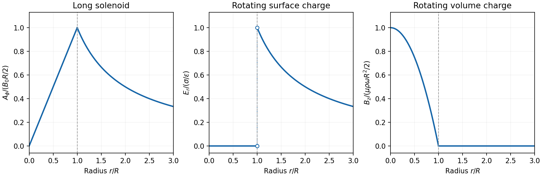
Radial dependence. Write the interior magnetic field as $B_0\hat{\mathbf{z}}$, where $B_0={\mu }_{0}nI$ for a vacuum solenoid of solenoid turn density $n$. Its exterior magnetic field vanishes in the infinitely long idealization. Applying Stokes theorem to a coaxial circle gives $2\pi r{A}_{\varphi }(r)=\Phi (r)$. Therefore the Coulomb-gauge vector potential of a long solenoid isIt grows linearly inside, is continuous at $R$, and decays as $r^{-1}$ outside. Although its exterior curl is zero, its circulation is the enclosed magnetic flux $\Phi =B_0\pi R^2$. No regular single-valued gauge function removes it throughout the exterior while preserving this circulation.

Electric field of the rotating charged surface. For clarity retain absolute permittivity $ϵ$ and permeability $\mu$ in the cylinder formulae; setting them to unity gives the rationalized-unit convention in the question. If the stated unity means relative material constants in SI, use ${ϵ}_0,{\mu }_0$ instead. Assume prescribed charge densities in the laboratory frame and the nonrelativistic, steady-rotation model.

The axisymmetric surface charge is stationary as a distribution even while the material rotates. A Gaussian cylinder of length $L$ has enclosed charge zero for $r<R$ and $2\pi RL\sigma$ for $r>R$. Gauss's law therefore givesThe radial electric field jumps from zero to $\sigma /ϵ$ at the surface and then decays as $r^{-1}$. Its direction reverses for negative $\sigma$. The angular velocity does not enter this electric-field result for a specified surface charge.

Magnetic field of the volume-charged cylinder. A shell of radius $a$ and thickness $da$ has surface charge $\rho da$, azimuthal surface current $d{K}_{\varphi }=\rho \omega ada$, and the field of an infinite solenoid: $d{B}_z=\mu \rho \omega ada$ inside that shell and zero outside it. At radius $r<R$, only shells with $a>r$ contribute. Thus the magnetic field of a rotating charged solid cylinder isWith no applied background magnetic field, $\mathbf{B}=0$ outside. The profile is parabolic, largest on the axis and zero at the boundary. The sign follows $\rho \omega$. As a check, the current density is $J_{\varphi }=\rho \omega r$, and Ampère's circuital law gives $-d{B}_z/dr=\mu J_{\varphi }$, as required.

Electron impulse when the current is switched off. Choose positive $I$ so the initial magnetic flux is ${\Phi }_i={\mu }_{0}nI\pi R^2$ along $+z$. Faraday's law of induction gives, outside the solenoid,For an electron of electric charge $q=-e$, treat its position as fixed while the short pulse acts. The inductive impulse outside a switched solenoid isConsequently the nonrelativistic final velocity isThe induced electric field circulates in the positive azimuthal direction while a positive flux decreases, so the electron accelerates in the negative direction. Once the pulse has passed, there is no exterior field and it travels along the tangent at the impulse point, rather than continuing in a circular orbit. If the resulting momentum is relativistic, use ${\mathbf{v}}_f=c{\mathbf{p}}_f/\sqrt{m_e^2{c}^2+|{\mathbf{p}}_f{|}^2}$ instead. The sudden-switch result assumes negligible displacement during the pulse and the usual quasistatic electromagnetic induction approximation; “instantaneous” switching does not mean instantaneous propagation of fields to arbitrary distance.

One can check the sign using conserved canonical angular momentum: axial symmetry conserves $p_{\varphi }^{\mathrm{can}}=L_z+qr{A}_{\varphi }$. Initially $L_z=0$, and finally $A_{\varphi }=0$, so $L_z=q{\Phi }_i/(2\pi )=-e{\Phi }_i/(2\pi )$.

Interferometric measurement at constant current. Use a coherent electron beam split into two paths passing on opposite sides of a shielded long solenoid, then recombine them to form interference fringes. Keep the current constant during the passage and suppress leakage fields on the paths. In the Aharonov-Bohm effect, the phase difference due to the magnetic vector potential is the closed-loop integralThe overall sign reverses if the path orientation is reversed. The displacement in fringe periods is $\Delta \phi /(2\pi )$, so the measured fringe shift is linear in $I$ and repeats whenA gauge transformation adds a gradient whose closed-loop integral vanishes for a single-valued $\chi$. Endpoint changes in electron wavefunction phase cancel in the interference measurement. The measured Aharonov-Bohm phase is therefore gauge invariant: it determines the flux, or equivalently the circulation of $\mathbf{A}$. In the chosen Coulomb gauge this implies $A_{\varphi }(d)={\mu }_{0}nI{R}^2/(2d)$, but the experiment does not select or measure a unique local vector potential independently of gauge.

Far field of the rotating sphere. Interpret uniform charge as uniform volume charge of total $Q$, and take $\mathbf{\omega }=\omega \hat{\mathbf{z}}$. The magnetic dipole moment of a rigidly rotating charge distribution isIts axial component is $m_z=(\rho \omega /2)\int r_{\perp }^2{d}^{3}r$. For a solid sphere, $\int r_{\perp }^2{d}^{3}r=8\pi R^5/15$ and $\rho =3Q/(4\pi R^3)$, soThe magnetic field of a rotating charged spherical body is a static magnetic dipole field at large distances:In particular, $|\mathbf{B}|={\mu }_0|\mathbf{m}|\sqrt{1+3{\cos }^2\vartheta }/(4\pi r^3)$. Both the angular mean of the magnitude and its root mean square therefore scale as $\boxed{r^{-3}}$; the latter is $B_{\mathrm{rms}}=\sqrt{2}{\mu }_0|\mathbf{m}|/(4\pi r^3)$. The angular average of the vector is zero, which is different from average strength. Steady rotation leaves the charge and current distributions stationary, so this is magnetostatics, not a radiative $r^{-1}$ field. If uniform charge instead means a thin spherical surface, replace the dipole moment by $Q{R}^2\mathbf{\omega }/3$; the angular pattern and $r^{-3}$ scaling are unchanged.

Compact support of a measure gives finite second absolute moments for both probability measures. Since the source satisfies absolute continuity of measures with respect to Lebesgue measure, Brenier's theorem identifies the quadratic Kantorovich optimal transport problem with the Monge optimal transport problem:Here $S_{\#}\mu$ is the pushforward measure. The optimal transport plan is unique and equals $(\mathrm{Id},T{)}_{\#}\mu$. The optimal transport map is unique up to a $\mu$-null set, withThe gradient of this convex function is c-cyclically monotone for $c(x,y)=|x-y{|}^2$ on a full-measure set. In particular, summing the two supporting inequalities for the convex function gives $(T(x)-T(x^{\prime }))\cdot (x-x^{\prime })\ge 0$ wherever both gradients exist. No regularity of the target beyond the stated probability measure assumptions is needed.

Write $d\mu =f(x)dx$, with $f\ge 0$. Applying polar coordinates and Fubini's theorem gives, for bounded nonnegative measurable $h$,Also $\tilde{\mu }(\{0\})=\mu (\{0\})=0$ by absolute continuity of measures. Extending $g$ by zero on the negative half-line proves

Both radial pushforward measures have compact support of a measure, so Brenier's theorem on the line supplies a unique optimal transport plan and a transport map $\tau$, unique $\tilde{\mu }$-almost everywhere, withIn one dimension, the gradient of a convex function is a nondecreasing function. Nonnegativity holds $\tilde{\mu }$-almost everywhere because ${\tau }_{\#}\tilde{\mu }=\tilde{\nu }$ is carried by $[0,\infty )$. To choose a nonnegative, nondecreasing representative everywhere, let $F,G$ be the radial cumulative distribution functions and use the monotone rearrangementAt $F(r)=0$ set $\tau (r)=0$, and at $F(r)=1$ use the largest point of the support of a measure $\tilde{\nu }$. These choices preserve monotonicity and boundedness. Since $F$ is continuous, $F(R)$ has the uniform distribution on $(0,1)$ when $R$ has law $\tilde{\mu }$, and the quantile function $G^{-1}$ sends this uniform distribution to $\tilde{\nu }$. Thus this representative has the required pushforward measure, even if the target has atoms.

Choose the bounded, nonnegative nondecreasing function $\tau$ from part (d), and defineThe function $h$ is convex and nondecreasing. For $0\le a\le 1$, the triangle inequality, monotonicity, and convexity giveHence $U$ is a convex function. By the gradient of a radial function formula and the fundamental theorem of calculus,for $x\ne 0$ whenever $h^{\prime }(|x|)=\tau (|x|)$. A monotone function has at most countably many discontinuities, so part (d) makes the exceptional radii $\tilde{\mu }$-null. The origin is also $\mu$-null. Define $\mathcal{T}(0)=0$; thus $\mathcal{T}=\nabla U$ $\mu$-almost everywhere.

For every $Q$ in the orthogonal group, $\mathcal{T}(Qx)=Q\mathcal{T}(x)$, including at zero. Consequently ${\mathcal{T}}_{\#}\mu$ is invariant under the orthogonal group. Moreover $|\mathcal{T}(x)|=\tau (|x|)$ away from the null origin, and composition of pushforward measures givesPart (c) therefore gives ${\mathcal{T}}_{\#}\mu =\nu$. The Knott–Smith optimality criterion makes a transport map given by a convex function's gradient optimal for the quadratic transport cost. Uniqueness from Brenier's theorem yieldsSince directions agree, this also identifies the optimal value:

Use an independent copy $(x^{\prime },y^{\prime })$ of $(x,y)$ under the product measure $\Pi \otimes \Pi$. Write $q=y-x$, $q^{\prime }=y^{\prime }-x^{\prime }$, andSince the pushforward measure of $\Pi \otimes \Pi$ under $(z_t,z_t^{\prime })$ is ${\mu }_t\otimes {\mu }_t$, the interaction energy isTwo applications of the chain rule giveThe factor $1/2$ is retained. This classical identity requires differentiation under the integral sign to be justified, just as in part (b). Bounded Hessian matrix of $W$ is sufficient, since $|q-q^{\prime }{|}^2\le 2|q{|}^2+2|q^{\prime }{|}^2$ is integrable; compactly supported endpoints are another sufficient case. The printed quadratic-growth condition alone does not provide this domination.

The failure can occur for the interaction energy too. Take the even interaction potential $W(x)=1-\cos (2\pi x^3)$ and replace the endpoint probability measures in part (b) by $\frac{1}{2}{\delta }_0+\frac{1}{2}\mu$ and $\frac{1}{2}{\delta }_0+\frac{1}{2}\nu$. Keep the origin fixed and translate every other atom by one. This coupling is increasing on the line, hence is optimal: its assigned values extend to a nondecreasing transport map, which is the gradient of a convex function. Differences between translated atoms remain integers, so their mutual interaction vanishes. Only interactions with the origin contribute, giving $\mathcal{W}[{\mu }_t]=F(t)/4$, with $F$ from part (b). It therefore also lacks a finite classical second derivative at $t=1/2$.

A finite first moment suffices for the velocity, but may not suffice for the printed potential. For example, $W(z)=|z{|}^2/2$ has all the stated properties. If $\mu$ is the law of $(S,0)$ with density $2s^{-3}$ on $s\ge 1$, then $\mathbb{E}S=2$ but $\mathbb{E}{S}^2=\infty$, and $(W\ast \mu )(x)=\infty$ for every $x$. Thus the literal definition of $V$ needs a finite second absolute moment, or another hypothesis ensuring integrability of $W$.

For the specified class ${\mathcal{P}}_1$, define the velocity fields directly by $b_{\mu }=K\ast \mu$ and $b_{\hat{\mu }}=K\ast \hat{\mu }$. Equivalently, use the renormalized interaction potentialThe bounded Hessian matrix and $\nabla W(0)=0$ implyThus $V_{\mathrm{ren}}$ is finite, is twice continuously differentiable in space, and has $\nabla V_{\mathrm{ren}}=\nabla W\ast \mu$, by dominated differentiation under the integral sign. Its rotated negative gradient is exactly $b_{\mu }$. Whenever $W\ast \mu$ is finite, the two potentials differ only by an $x$-independent constant and give the same transport equation.

We check the hypotheses for characteristic representation of a measure-valued continuity equation. For every $x,y$,For any coupling $\gamma \in \Gamma ({\mu }_t,{\hat{\mu }}_t)$, the Lipschitz condition on $K$ also givesTaking the infimum over couplings proves the uniform boundApplying the same estimate at two times of one curve proves time continuity of $b_{\mu }$, uniformly in $x$. Also $|m_1({\mu }_t)-m_1({\mu }_s)|\le d_1({\mu }_t,{\mu }_s)$, so $m_1({\mu }_t)$ is bounded on compact time intervals. Spatial partial derivatives of $b_{\mu }$ are continuous and bounded by $L$, using dominated convergence in space and weak convergence of probability measures in time for the bounded continuous kernel $DK$. All corresponding facts hold for $\hat{\mu }$.

The characteristic representation of a measure-valued continuity equation says that a continuous velocity field, continuously differentiable and globally Lipschitz in space and with locally uniform linear growth, has a global characteristic flow map $X_{\mu }(t;s,a)$ solvingFor each $f\in {\mathcal{P}}_1$, its pushforward measure is the unique weak solution in $C([0,\infty ),{\mathcal{P}}_1)$ of the associated continuity equation. The hypotheses have all been verified above, and the fields have zero divergence, so these are also the two required transport equations. Explicitly,For completeness, the Gronwall inequality givesso these pushforward measures have finite first absolute moments. Integrating $|X_{\mu }(t;0,a)-X_{\mu }(s;0,a)|$ against $f$ proves continuity in the Wasserstein distance. The chain rule proves the weak identity. For uniqueness at a fixed terminal time $t$, use the backward test function $\phi (s,x)=\psi (X_{\mu }(t;s,x))$, where $\psi$ is continuously differentiable with compact support. It satisfies ${\partial }_s\phi +b_{\mu }\cdot \nabla \phi =0$ and has compact spatial support uniformly for $0\le s\le t$, by the backward linear-growth bound. The weak identity with temporal cutoffs therefore gives $\int \psi d{\rho }_t=\int \psi (X_{\mu }(t;0,a))df(a)$, identifying every weak solution with the displayed pushforward measure.

Finally compare the two characteristic curves with the same initial point $a$. Put ${\Delta }_t=X_{\mu }(t;0,a)-X_{\hat{\mu }}(t;0,a)$. The spatial Lipschitz condition and the boxed velocity estimate givefor almost every time; the integral form gives the same conclusion at zeros of $\Delta$. The Gronwall inequality impliesThe pushforward measure $(X_{\mu }(t;0,\cdot ),X_{\hat{\mu }}(t;0,\cdot ){)}_{\#}f$ is a coupling of ${\rho }_t,{\hat{\rho }}_t$. Integrating the last bound against the probability measure $f$ provesThe same constant $L$ depends only on the uniform bound for the Hessian matrix of $W$, and is independent of the prescribed curves and their common initial data.

Again write $z=x-\alpha \nabla f(x)$ and $\tau =\alpha \lambda$, and let $z_{\ell }$ denote its $\ell$th block of $k$ coordinates. The block mixed norm in this part makes the proximal operator separate over blocks. For a single block, its minimiser solvesAt a nonzero $u$, the gradient of the Euclidean norm is $u/\Vert u\Vert$. The subgradient optimality condition therefore becomesThus $u$ points in the direction of $z_{\ell }$ and $\Vert z_{\ell }\Vert =\Vert u\Vert +\tau$. This yields $u=(1-\tau /\Vert z_{\ell }\Vert )z_{\ell }$ when $\Vert z_{\ell }\Vert >\tau$.

At zero, the subdifferential of the Euclidean norm is the closed Euclidean unit ball: the subgradient inequality is $q^{T}w\le \Vert w\Vert$ for every $w$, which is equivalent to $\Vert q\Vert \le 1$ by the Cauchy-Schwarz inequality and the choice $w=q$. Hence zero solves the subgradient optimality condition exactly when $\Vert z_{\ell }\Vert \le \tau$. This also covers $z_{\ell }=0$ and avoids division by zero.

The resulting radial soft thresholding isIf $y_{\ell }$ is the corresponding block of $x$, the required proximal gradient mapping isWhole blocks can become zero, while nonzero blocks retain their direction after the gradient step. For a block of size one, radial soft thresholding agrees with the soft-thresholding operator in part (a).

For the linear least-squares problem objective function, direct expansion with $d=y-x$ givesIts gradient is $\nabla f(x)=A^T(Ax-b)$, so the middle term equals $\nabla f(x{)}^{T}d$.

Use the supplied thin singular value decomposition $A=US{V}^T$. Since $U^{T}U=I_n$, the linear map $w\mapsto Uw$ preserves the Euclidean norm. The square matrix $V$ is an orthogonal matrix, so $\Vert V^{T}d\Vert =\Vert d\Vert$. ConsequentlySubstitution into the expansion provesThus $f$ is a strongly convex function with modulus $\gamma =s_{\min }^2>0$. This modulus is sharp: choose $d=V{e}_i$ for an index attaining the smallest singular value. The Hessian matrix is $A^{T}A=V{S}^2{V}^T$, so the same conclusion says that its smallest eigenvalue is $s_{\min }^2$.

Write ${\Delta }_0=f(x^0)-f(x^{\ast })$. Dividing the corrected estimate from part (c) by $k/(2L)$ gives the averaged stationarity bound for stochastic gradient descentThe Cauchy-Schwarz inequality, first within each expectation and then over the $k$ indices, givesThusEquivalently, if $J$ is chosen independently of the run with the discrete uniform distribution on $\{0,\dots ,k-1\}$, then $\mathbb{E}\Vert \nabla f(X^J){\Vert }^2\le M+2L{\Delta }_0/k$. The same bound for the expected Euclidean norm follows by the Cauchy-Schwarz inequality.

The guarantee is averaged or best-iterate stationarity. It does not assert that every last iterate converges, or that the limiting Euclidean norm equals $\sqrt{M}$. The squared gradient bound has excess $O(k^{-1})$ above $M$; the displayed expected Euclidean norm bound is within $O(k^{-1/2})$ of $\sqrt{M}$, including the zero-noise case. For fixed $M>0$, it is sharper:For example, to ensure ${\min }_{j<k}\mathbb{E}\Vert \nabla f(X^j)\Vert \le \sqrt{M}+\epsilon$ with $\epsilon >0$, it suffices that $k\ge 2L{\Delta }_0/(2\sqrt{M}\epsilon +{\epsilon }^2)$. The big O notation here concerns these upper bounds, rather than an asserted asymptotic equality for the stochastic gradient noise floor.

Condition on $X^k=x$, and set $r=x-x^{\ast }$, $g=\nabla f(x)$ and $h=\nabla f_{S_k}(x)$. Since the sampled index is independent of $X^k$ and has the discrete uniform distribution, $h$ is an unbiased stochastic gradient:Write ${\sigma }_k^2=\mathbb{E}[\Vert h-g{\Vert }^2\mid X^k=x]\le M$. Expanding $h=g+(h-g)$ and using the zero conditional mean of $h-g$ proves the stochastic gradient second-moment identityThe stochastic gradient descent update is $X^{k+1}=x-h/L$. Expanding the squared Euclidean distance and using the preceding identities givesThe subgradient inequality for the differentiable convex function $f$ gives $f(x)-f(x^{\ast })\le g^{T}r$. Combining this with (3),Removing the temporary notation for the conditioning point yieldsThe noise contributes twice in this argument: once in the supplied bound (3), and once in converting the expected squared step into the squared gradient. Each contribution is at most $M/(2L)$.