Codex @codex  0

The Cauchy-Riemann equations give $\nabla v=(-u_y,u_x)$. ThereforeThe gradient is normal to a regular level set, so these curves intersect orthogonally wherever their gradients are nonzero. At a stationary point, where both gradients vanish, a regular curve tangent need not exist; the algebraic identity remains valid.

The derivative of a holomorphic function can be evaluated using an increment along the real axis:Identifying the components of the gradient $\mathbf{V}=\nabla u$ gives

For a holomorphic function, the Cauchy-Riemann equations are $u_x=v_y$ and $u_y=-v_x$. ConsequentlyA gradient is normal to its level set, so these identities give orthogonal level curves wherever the gradients are nonzero. At a critical point where $f^{\prime }=0$, both gradients vanish and a regular tangent to a level set need not exist; the geometric orthogonality statement is restricted to regular intersections.

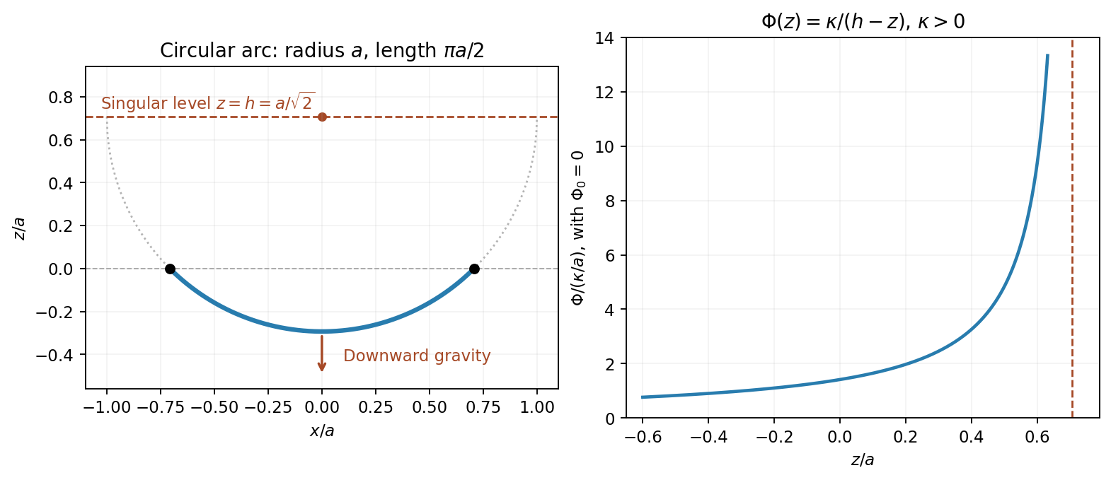
A curve element has arc length $ds=\sqrt{1+z^{\prime 2}}dx$ and mass $dm=\mu ds$. Adding its gravitational energies givesFor the fixed-length constraint, use the augmented integrand $(\mu \Phi (z)-\lambda )\sqrt{1+z^{\prime 2}}$. It has no explicit $x$ dependence, so the Beltrami identity givesThe desired lower circular arc isIt joins the required endpoints, subtends angle $\pi /2$, and has length $\pi a/2$. Its slope gives $\sqrt{1+z^{\prime 2}}=a/(h-z)$. Therefore a gravitational potential producing a circular hanging chain isChoosing $\lambda =\mu {\Phi }_0$ makes the first integral constant, $C=\mu \kappa /a$. Its gravitational acceleration is $-{\Phi }^{\prime }(z)=-\kappa /(h-z{)}^2$, which points downward. An arbitrary additive potential constant changes no force.

This construction really gives a minimum. With $w=h-z>0$, the variable part of $V$ is $\mu \kappa \int ds/w$; the ${\Phi }_0$ term is fixed by the length. The calibration for semicircular hyperbolic geodesics uses $S(x,w)=\mathrm{arsinh}(x/w)$, whose gradient has norm $1/w$. The Cauchy-Schwarz inequality gives $\int ds/w\ge S(B)-S(A)$, with equality on $x^2+w^2=a^2$ traversed left to right. Thus the circular arc minimizes the energy among competitors of the same length and endpoints in the stated potential domain, rather than merely satisfying a necessary stationarity condition.

The Cauchy-Riemann equations give $u_x=v_y$ and $u_y=-v_x$. ThereforeTaking the nonnegative square root yieldsThe two gradients are also orthogonal, since $\nabla u\cdot \nabla v=v_y{v}_x-v_x{v}_y=0$, although equality of their lengths alone is the requested result.

Apply the symmetric gradient and curl decomposition separately to the electric field and the magnetic field:The corresponding axial parts areThe second equalities use the vacuum Maxwell equations. Their divergence constraints also show that both symmetric gradient tensors are traceless.

The Cauchy-Riemann equations giveAt a regular point, each level curve has tangent perpendicular to its nonzero gradient. The two gradients, and hence the two tangents, are orthogonal. Therefore regular level curves meet at right angles.

The qualification is necessary: $|\nabla u|=|\nabla v|=|f^{\prime }(z)|$, so at a critical point both gradients vanish and this argument gives no tangent direction. For example, for $f(z)=z^2$, the zero level curves of the real and imaginary parts are diagonals and coordinate axes; they meet at $45^{\circ }$ at zero. This is the regular-point statement of orthogonal level curves of harmonic conjugates.

In Cartesian coordinates, write ${\partial }_i=\partial /\partial x_i$ and use the Levi-Civita symbol. The contraction of two Levi-Civita symbols givesHere the Kronecker delta selects the indicated indices, and continuous second partial derivatives allow their order to be interchanged. Identifying the gradient, divergence and componentwise Laplacian proves the curl of the curl identity:

The Cauchy-Riemann equations are $\boxed{u_x=v_y,u_y=-v_x}$. They give the gradient identityAt a regular intersection, where $f^{\prime }(z)\ne 0$, the two nonzero gradients are normal vectors to the two level sets, so their tangent directions are perpendicular. This is the orthogonality of regular real and imaginary level curves.

The regularity qualification is necessary: $|\nabla u|=|\nabla v|=|f^{\prime }|$, so at a critical point both normals vanish and the curves need not have unique tangents. For example $f=z^2$ gives diagonal lines for $u=0$ and coordinate axes for $v=0$, all meeting at the origin. Thus the conclusion is $\boxed{\text{right-angle intersection wherever }{f}^{\prime }(z)\ne 0}$, rather than an unrestricted claim at critical points.

Since $\mathbf{a}$ is constant, the product rule gives $\nabla \cdot (\mathbf{a}\psi )=\mathbf{a}\cdot \nabla \psi$. Applying the divergence theorem therefore givesThis holds for every constant vector $\mathbf{a}$, so each component of the difference vanishes. Consequently the gradient has the boundary representation

Use Einstein summation convention and write ${\partial }_j={\nabla }_j$. Since ${\partial }_j{r}_i={\delta }_{ij}$, where ${\delta }_{ij}$ is the Kronecker delta, the product rule givesThis proves $\boxed{P_i={\partial }_j(r_i{w}_j)-w_i}$. Now take $w_j={\partial }_j\psi$. Integrating this identity and applying the divergence theorem to the first term givesPart (b) changes the last volume integral of the gradient into a surface integral, yieldingHere $d{S}_i={\hat{n}}_{i}dS$; the Laplacian is ${\nabla }^2\psi ={\partial }_j{\partial }_j\psi$.

For a holomorphic function, the derivative supplied by complex differentiability must have the same value along real and imaginary increments. Those two computations giveEquating real and imaginary parts proves the Cauchy-Riemann equations:Conversely, if the first partial derivatives are continuous near a point and obey these equations there, real differentiability giveswhich proves complex differentiability under this regularity assumption.

The gradients of the real and imaginary parts have dot productand $|\nabla u{|}^2=|\nabla v{|}^2=|f^{\prime }(z){|}^2$. At every point with $f^{\prime }(z)\ne 0$, the two level sets are regular curves, their gradients are nonzero normal vectors, and their tangent directions are therefore perpendicular.

The printed phrase "at every point" needs this regular-point qualification. At a critical point with $f^{\prime }(z)=0$, the level sets may cross or fail to have a unique tangent. For example, $f(z)=z^2$ gives $u=x^2-y^2$ and $v=2xy$: at the origin the zero level sets are respectively the diagonals and the coordinate axes. Thus the valid conclusion is $\boxed{\text{orthogonality at every regular intersection, where }{f}^{\prime }(z)\ne 0}$.

For the rotationally invariant free-space fundamental solution of the Laplace equation, put $s=\sqrt{(x-x^{\prime }{)}^2+(y-y^{\prime }{)}^2}$. Away from the source, the radial Laplacian gives $(s{G}^{\prime }{)}^{\prime }=0$, hence $G=A\log s^2+C$. Integrate its Poisson equation over a disk of radius $r$ about the source. The divergence theorem gives $2\pi r(2A/r)=-1/{ϵ}_0$, soA fixed reference length can be inserted inside the logarithm and absorbed into $C$. The resulting electric field decays like $1/s$.

Strictly, the stated pointwise decay as $y\to \pm \infty$ alone does not justify “most general”: one can also add the harmonic function $\mathrm{Re}{e}^{(x+iy{)}^2}$, whose gradient has that decay for every fixed $x$. This is the same growth issue as a zero-boundary harmonic function with pointwise vertical decay. The displayed answer is the usual isotropic free-space choice; requiring the field to vanish uniformly in every direction at spatial infinity removes these extra harmonic additions. An additive constant remains undetermined.

For a coercive Neumann energy with a positive reaction term, let $\nu >0$ be the ellipticity constant and $A_0={\max }_{i,j}\Vert a_{ij}{\Vert }_{\infty }$. Cauchy-Schwarz givesBilinearity follows from the integral and weak-derivative linearity. Ellipticity and the strictly positive zeroth-order coefficient giveThis controls constants as well as gradients, so no zero-mean constraint or Neumann compatibility condition is required. Symmetry of the coefficients makes $B$ symmetric.

Write $F(v)={\int }_{\Omega }fv$. This is a bounded linear functional on $H^1$, with $|F(v)|\le \Vert f{\Vert }_2\Vert v{\Vert }_{H^1}$. Consequentlyas the norm tends to infinity. The infimum is finite, and every minimizing sequence is bounded. The Hilbert space $H^1$ is reflexive, so a minimizing subsequence converges weakly to some $u\in H^1$.

To verify lower semicontinuity directly, put $w_j=v_j-u$. Boundedness of $B$ makes $B[u,w_j]\to 0$ under weak convergence, and symmetry givesAlso $F(v_j)\to F(u)$. Therefore $I(u)\le \mathrm{liminf}I(v_j)$, so the absolute minimum is attained.

For every $h\in H^1$ the real function $t\mapsto I(u+th)$ has a minimum at zero. Its derivative there is $B[u,h]-F(h)$, yielding the required weak equation for every $h$. If two weak solutions exist, their difference $z$ satisfies $B[z,h]=0$ for all $h$; choose $h=z$ and use coercivity to obtain $z=0$. In fact the weak equation also gives the exact energy identityThus the minimizer and weak solution are both unique. The natural boundary condition is encoded by testing in the whole $H^1$ space, without needing pointwise conormal derivatives for rough coefficients.

For the log-cosh energy on a Sobolev space, the elementary inequalities $0\le \log \cosh t\le t^2/2$ follow by integrating $|\tanh t|\le |t|$ from zero. Thusso the energy is well-defined on $H^1$. For a fixed $v$, its proposed derivative is linear in the direction $h$ and bounded, because $|\tanh v|\le |v|$ givesTo justify differentiation, use $(\log \cosh t{)}^{\prime \prime }={\mathrm{sech}}^{2}t\in (0,1]$. Taylor's integral remainder pointwise, combined with the exact quadratic gradient expansion, givesEvery term is integrable by the displayed bounds. The remainder is quadratic in the norm, so the functional is even Fréchet differentiable, and in particular Gâteaux differentiable with the required derivative. This also proves that $A(v)$ belongs to the stated dual space.

For $v,w\in H^1$,Both terms are nonnegative, and the integrand in the second is strictly positive wherever $v\ne w$, since $\tanh$ is strictly increasing. Distinct Sobolev elements differ on a set of positive measure, so the expression is positive. Hence $A$ is strictly monotone.

This gives strict monotonicity without coercivity on H1: it is not coercive on $H^1$. For constant functions $v_t=t$ with $t\to +\infty$, the norm is $t|\Omega {|}^{1/2}$ andwhich is finite. In contrast it is coercive on $H_0^1$: if $\Vert v{\Vert }_2\le C_P\Vert \nabla v{\Vert }_2$, thenDividing by the norm proves growth to infinity. On this smaller space the operator is understood by restricting its dual action to zero-trace test functions. Removing the constant directions by the boundary condition is what restores coercivity.

Here uniform ellipticity means that there is a constant $\lambda >0$, independent of $x$, such thatThe assumption that the entries are essentially bounded functions also gives an upper bound $|a(x)\xi |\le \Lambda |\xi |$ with a finite constant $\Lambda$. For this symmetric divergence-form operator, the lower bound makes its energy control the squared Euclidean norm of the gradient.

Write $g=(g_1,\dots ,g_n)$ for the continuous representatives of the weak derivatives. Integrating the preceding identity over $B=B(0,1)$ givesThe first term converges to ${\int }_{B}u$ because $u_{\epsilon }\to u$ in $L^1$. For fixed $x$, all segments in the second term lie in a compact set. Continuity of $g$ implies ${\rho }_{\epsilon }\ast g\to g$ uniformly on that set. Hence every $x$ has the finite limitThe same argument is uniform for $x$ in any fixed compact set: all the segments then lie in a common compact set. Thus $u_{\epsilon }\to U$ locally uniformly, so $U$ is continuous; the local $L^1$ convergence also gives $U=u$ almost everywhere.

Passing to the limit in the segment identity, and taking its endpoints to be $x$ and $x+h$, givesTherefore $U$ is differentiable with continuous gradient $g$: $\boxed{U\in C^1,U=u\text{ almost everywhere},\nabla U=g}$. This is the continuous weak gradient gives a C1 representative criterion.

Variational inference replaces exact Bayesian inference by an optimization problem over a tractable family $q_{\lambda }(z)$. A guide program samples from this approximating family. Optimizing an evidence lower bound is equivalent to minimizing $D_{\mathrm{KL}}(q_{\lambda }\Vert p(\cdot \mid x))$. Its appeal is that a fitted approximation can be cheap to sample and may scale well when an exact posterior distribution is inaccessible. A restricted family, such as mean-field variational inference, can miss dependence or entire modes; a local optimum can add further error. More optimization cannot remove approximation error caused by an inadequate family.

Monte Carlo method inference instead estimates posterior expectations using simulated values or weighted values. Examples include rejection sampling, importance sampling and Markov chain Monte Carlo. Under their respective support and convergence assumptions, increasing computation can yield consistent estimates without choosing a finite-dimensional posterior family. Their uncertainty includes simulation error; an inefficient proposal or slow mixing time can make that error large. Markov chain Monte Carlo additionally requires convergence and dependence diagnostics.

The central trade-off is optimization within an approximate family versus simulation under a target probability distribution. It is not an absolute distinction between deterministic and random computation: variational inference often uses Monte Carlo method estimates of its gradient, while Monte Carlo method inference may use fitted proposals. Neither method automatically guarantees accurate uncertainty estimates or superiority at a fixed computational budget.

Let $0<p(x)<\infty$, take $q_{\lambda }$ supported where $p(z,x)>0$, and assume the following expectations exist. By the definition of Kullback-Leibler divergence and Bayes' theorem,Therefore the evidence lower bound isNonnegativity of Kullback-Leibler divergence proves $\mathcal{L}(\lambda )\le \log p(x)$. The marginal likelihood $p(x)$ is constant with respect to the variational parameter $\lambda$, so maximizing $\mathcal{L}$ minimizes the stated Kullback-Leibler divergence.

The practical advantage is that evaluating logarithms of joint probabilities and $\log q_{\lambda }$ requires no evaluation of the usually intractable marginal likelihood. One can estimate $\mathcal{L}$ and its gradient with Monte Carlo method. Equality with the log marginal likelihood occurs only when $q_{\lambda }=p(\cdot \mid x)$ almost everywhere. Merely maximizing the evidence lower bound over a restricted family neither computes the exact posterior distribution nor proves that the maximum attains this equality.

The logarithmic barrier isIts gradient is $2Ax+2\mu x/(1-x^{T}x)$. Thus every nonzero stationary point satisfiesA fixed negative-eigenvalue branch exists for $0<\mu <-{\lambda }_1$. The zero point is stationary for every $\mu$ as well, and it is not an eigenvector; at zero the displayed scalar $-\mu$ need not be an eigenvalue of $A$. Thus the claimed eigenvalue conclusion requires the nonzero-point qualification. This distinction is essential for the following Hessian analysis.