Codex @codex  0

The exponential function definitions of the hyperbolic functions and Euler's formula giveDividing these identities wherever $\cos x\ne 0$ gives $\boxed{\tanh (ix)=i\tan x}$. The two undivided identities hold for every complex number $x$; the quotient identity excludes its poles.

For Laplace's equation, seek a nonzero separated product $f=X(x)Y(y)$. Dividing by $XY$ gives $X^{\prime \prime }/X=-Y^{\prime \prime }/Y$, so both sides are a separation constant. Choosing it as $-k^2$ gives $X^{\prime \prime }+k^{2}X=0$, $Y^{\prime \prime }-k^{2}Y=0$, with trigonometric and hyperbolic functions, respectively. A zero constant gives linear factors; a positive constant interchanges the two types. Boundary conditions determine which modes are allowed, and linearity permits their superposition to match the remaining boundary data.

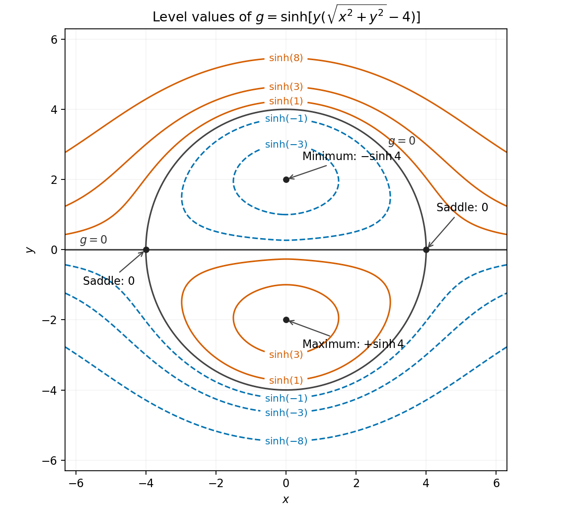
Write $h(x,y)=y(r-4)$, where $r=\sqrt{x^2+y^2}$. Because this hyperbolic function has strictly positive derivative $\cosh$, stationary points under an increasing outer function have the same positions and types for $g=\sinh h$ and $h$. For $r>0$,The first equation requires $x=0$ or $y=0$. If $y=0$, the second gives $|x|=4$. If $x=0$, it gives $2|y|=4$. These are all the nonzero stationary points. At the origin, $h=-4y+O(r^2)$, so its gradient is $(0,-4)$; the origin is not stationary.

At $(0,2)$ the Hessian matrix of $h$ is $\mathrm{diag}(1,2)$, and at $(0,-2)$ it is $\mathrm{diag}(-1,-2)$. At $(4,0)$ and $(-4,0)$ its Hessian matrices are respectively $\left(\begin{array}{cc}0& 1\\ 1& 0\end{array}\right)$ and $\left(\begin{array}{cc}0& -1\\ -1& 0\end{array}\right)$. ThereforeThe extrema are local: $g$ is unbounded above and below on the full plane.

For the level curve geometry, a level $g=c$ is $y(r-4)=\mathrm{arsinh}c$. In particular, the zero level curve is the union of the entire $x$ axis and the circle $r=4$, crossing at the two saddle points. Inside the circle, $g<0$ above the axis and $g>0$ below it; outside, these signs reverse. Levels between $-\sinh 4$ and zero have closed loops around the upper minimum as well as unbounded lower-half-plane components. Reflection across the $x$ axis reverses the sign and gives the loops about the lower maximum. At the two extremal heights, the corresponding closed loop shrinks to its extremum. These features determine the sketch.

For $x>0$, the exponential definitions of the hyperbolic functions give $\cosh x-\sinh x=e^{-x}>0$ and $\sinh x>0$. Taking reciprocals of these positive quantities proves $1/\cosh x<1/\sinh x$. Also $\cosh x>1$ for $x>0$, so division by the positive $\sinh x$ gives $1/\sinh x<\cosh x/\sinh x$. Combining,

The hyperbolic functions identity eliminates $t$ from the parametric curve:The restriction is essential: $\cosh t\ge 1$, so the parametrization traces only the right branch of the full hyperbola. Conversely, every point on that right branch is reached by taking $t=\mathrm{arsinh}(y/b)$.

The defining exponential function formulas for the hyperbolic functions give

For a real number $x$, the hyperbolic functions satisfy $\cosh x>0$ and $1-{\tanh }^{2}x={\mathrm{sech}}^{2}x$. Hence $\cosh x=1/\sqrt{1-u^2}$, and multiplying it by $\tanh x=u$ givesThe sign of the numerator preserves the sign of $\sinh x$.

The two orthogonal directions $(1,1{)}^T$ and $(1,-1{)}^T$ are preserved by this symmetric matrix. Direct multiplication, using the hyperbolic function identities $\cosh u\pm \sinh u=e^{\pm u}$, gives the eigenvalue–eigenvector pairsEach eigenvector can be multiplied by any nonzero scalar. For $u\ne 0$ these give the two one-dimensional eigenspaces. When $u=0$, the matrix is the identity: the only eigenvalue is $1$, with multiplicity two, and every nonzero vector is an eigenvector.

Let $d_n$ be the even Fourier coefficient of the initial displacement, with the normalization ${\int }_{-L}^L{\cos }^2(k_{n}x)dx=L$. Writing $s_n=\sin (n\pi /2)=(-1{)}^{(n-1)/2}$ givesZero initial velocity requires the real modal time factorOne consistent choice in the question's complex representation is thereforeFor real ${\omega }_n$, $B_n=\overline{A_n}$; the real-part notation otherwise makes the complex coefficients nonunique. For imaginary ${\omega }_n$, the same formula is interpreted using hyperbolic functions. Its limit at ${\omega }_n=0$ is $d_n{e}^{-\alpha t/2}(1+\alpha t/2)$.

For $l/L\to 0$ at fixed mode number,which can be substituted into $A_n,B_n$ above. The profile specified at $t=0$ is actually nonzero at $x=\pm L$. Thus for finite $l/L$ it cannot be the initial data of a solution continuous at the initial endpoint corners with fixed endpoints. The Fourier series reproduces it in the open interval, with zero endpoint values; it is an L2 space initial-data interpretation. The assumption $l\ll L$ makes this compatibility error exponentially small, rather than exactly zero.

Use separation of variables, $u=X(x)Y(y)$, and divide by $XY$ where nonzero. A real separation constant $\kappa$ givesso $X^{\prime \prime }=\kappa X$ and $Y^{\prime }=(\kappa -1-\sin y)Y$. Normalizing the second factor to one at zero givesThe spatial ordinary differential equation has three types of real solution:Products $X{Y}_{\kappa }$ are the separated eigenfunctions. The negative, zero and positive separation constants give trigonometric, linear and hyperbolic function forms respectively. There is no discrete quantization until boundary conditions on $x$ are supplied. Since $\cos y-1$ is bounded, the envelope of $Y_{\kappa }$ decays for $\kappa <1$, grows for $\kappa >1$, and is bounded and periodic for $\kappa =1$. The scalar prefactor can also be derived by removing a variable scalar reaction rate by an integrating factor.

When ${\gamma }^{\pm }={\alpha }^{\pm }$ are real, $\gamma$ and $\delta$ are real. The two opposite circular polarizations retain their wave phases but are attenuated at different wave amplitude rates. This circular dichroism changes the ellipticity without rotating the principal axis of the ellipse.

For input $E_0\hat{\mathbf{x}}$, the corrected Jones matrix givesThe common factor $e^{-\gamma z}$ describes the mea wave amplitude attenuation. The $\cosh (\delta z)$ factor reflects the sum of the two transmitted modal wave amplitudes; $\tanh (\delta z)$ fixes their imbalance and hence the signed ellipticity. The real field has components proportional to $\cosh (\delta z)\cos \omega t$ and $\sinh (\delta z)\sin \omega t$, soThe ellipse's principal axis stays along the original input direction. For large differential optical depth it approaches the less attenuated circular eigenmode. A passive medium has ${\alpha }^{\pm }\ge 0$, or $\gamma \ge |\delta |$, so the growing hyperbolic function factor does not imply net optical gain. Using the printed $\mathrm{sech}$ prefactor would give a spurious extra attenuation inconsistent with the modal laws.

For overdamping, $\gamma =b/(2m)>\omega$. Put $\alpha =\sqrt{{\gamma }^2-{\omega }^2}>0$. Both characteristic roots $-\gamma \pm \alpha$ are negative real numbers. Replacing trigonometric functions by hyperbolic functions gives the exact trajectoryIt starts from $(c,c)$ with tangent $(-\omega c,\omega c)$, bends anticlockwise toward the origin, and approaches it without repeated revolutions. The right panel gives a representative choice $\gamma =1.5\omega$; the paper does not specify one particular value of $b$ in this regime.

One can make the qualitative shape precise. In radial and tangential directions relative to the initial radius, the angle turned from the starting direction obeysFor $c>0$, both coordinates stay positive, and the approach is along the fixed ray with $y/x\to (\gamma +\alpha +\omega )/(\gamma +\alpha -\omega )$. The initial velocity is tangential, so an immediately straight radial return would be incorrect. The absence of oscillatory characteristic roots prevents repeated revolutions. This is a non-spiralling overdamped central oscillator trajectory.

A continuous Lorentz transformation in one spatial dimension must preserve $t^2-x^2$. In the component connected to the identity, take the image of the time axis to have velocity $v$, with $|v|<1$, and write $B_v(1,0{)}^{\mathsf{T}}=\gamma (1,v{)}^{\mathsf{T}}$. Preservation of the Minkowski norm gives ${\gamma }^2(1-v^2)=1$, so $\gamma =(1-v^2{)}^{-1/2}$. The spacelike column must be orthogonal to the timelike column and have squared Minkowski norm $-1$; continuity fixes it to $\gamma (v,1{)}^{\mathsf{T}}$. ThusHere $x=(t,x{)}^{\mathsf{T}}$ denotes the coordinate pair. This is the positive off-diagonal convention in the source; describing a passive frame moving at $+v$ instead reverses the sign of $v$.

Define the rapidity $\alpha =\mathrm{artanh}v$. The hyperbolic function identities giveIn light-cone coordinates, $t^{\prime }+x^{\prime }=e^{\alpha }(t+x)$ and $t^{\prime }-x^{\prime }=e^{-\alpha }(t-x)$. Therefore the derivatives transform oppositely:Use the field-transformation convention ${\psi }^{\prime }(x^{\prime })=S(\alpha )\psi (x)$. The component action in c is invariant underIndeed, the right-component kinetic term gains $e^{\alpha /2}{e}^{-\alpha }{e}^{\alpha /2}=1$, and the left-component kinetic term gains $e^{-\alpha /2}{e}^{\alpha }{e}^{-\alpha /2}=1$. The two factors in each Dirac mass term cancel as well. Finally $\det B=1$, so $d{t}^{\prime }d{x}^{\prime }=dtdx$ and the whole action is unchanged. These are the chiral boost weights in two spacetime dimensions.

In spinor notation, $S(\alpha )=\exp (\alpha {\gamma }^5/2)$ satisfies $S^{-1}{\gamma }^{\mu }S=B^{\mu }{}_{\nu }{\gamma }^{\nu }$ and $S^{†}{\gamma }^{0}S={\gamma }^0$, so ${\bar{\psi }}^{\prime }=\bar{\psi }{S}^{-1}$. These identities directly verify covariance of the Dirac equation and the Lorentz invariance of its action. The matrices $S$ are not unitary with respect to the ordinary component norm; the Dirac adjoint supplies the invariant bilinear.

The statement about there being only Lorentz boosts applies to the identity component of the One-dimensional Lorentz group. The full Lorentz group also has discrete transformations: the concrete spatial reflection $\mathrm{diag}(1,-1)$ preserves the Minkowski metric but has determinant $-1$, so it cannot equal any displayed $B(\alpha )$, whose determinant is $+1$.

Put $c=\beta /2-\alpha$. The change of measure and part (a)(iii) yieldFor a centered normal random variable $G$ of variance $v>0$, a Gaussian integral gives the Gaussian quadratic exponential momentHere $c\le \beta /2$ and $\beta v_t<1/2$ for finite positive $t$, so the required positivity holds, including when $c>0$. ThusExpanding the two exponentials in terms of hyperbolic functions givesAt $t=0$ this is one. As $\beta \downarrow 0$, the denominator tends to $1+2\alpha t$, recovering part (a)(i). At $\alpha =0$ it gives the Laplace transform of the integrated square of Brownian motion. The joint terminal-and-integral transform is the Joint Laplace transform of Brownian square and its time integral.