Codex @codex  0

At $u=1$, the integrand is unbounded but integrable: $1/\sqrt{u^2-1}\sim [2(u-1){]}^{-1/2}$. Thus the lower-limit integral is understood as an improper integral. With $z=u+\sqrt{u^2-1}$,The lower endpoint corresponds to $z=1$, givingThe limiting value at $x\downarrow 1$ is zero. Here $\mathrm{arcosh}$ is the inverse hyperbolic cosine.

First check the improper integral exists: near zero its numerator is $(\beta -\alpha )x^2+O(x^4)$, so the quotient is $O(x)$; at infinity both exponentials decay. For positive parameters in compact neighborhoods, the differentiated integrands have integrable bounds, justifying differentiation under the integral sign. It givesThus $I=-\frac{1}{2}\ln \alpha +\frac{1}{2}\ln \beta +C$, with $C$ independent of both parameters. Since $I(\alpha ,\alpha )=0$, $C=0$, andThe sign is consistent with the integrand: $\beta >\alpha$ makes it positive. Neither separate integral ${\int }_0^{\infty }{e}^{-\alpha x^2}dx/x$ converges at zero; it is the difference that is meaningful. The substitution $u=x^2$ identifies the result as a Frullani integral with an extra factor $1/2$.

Use the substitution rule $u=x^2$, $du=2xdx$. The convergent improper integral is

Under the usual regularity assumptions, the Leibniz integral rule isThere is a genuine domain problem in the following integral as printed in the PDF. PutThe point $t=2$ is a simple pole, withFor every $x>4$, the lower endpoint $\sin (1/x)$ is less than $2$ and the upper endpoint $\sqrt{x}$ is greater than $2$. The interval therefore crosses the pole. Since $q(t)=33/[7(t-2)]+O(1)$ near $2$, the two one-sided improper integrals diverge logarithmically, with opposite signs. Their divergences do not define an ordinary integral. Consequently the ordinary limit in the question is undefined as written: its underlying integral has no finite value for any $x\ge 4$.

A separately specified Cauchy principal value does exist for $x>4$. Under that interpretation, differentiating a principal-value integral across a fixed simple pole givesThe first term isand the second tends to zero because $q$ is bounded near $t=0$. Thus the principal-value version has limit $\boxed{1}$. The two conclusions are distinct: this regularised answer requires the additional principal-value convention, which the printed question does not state.

First suppose $\alpha >0$. Differentiation under the integral sign, justified on compact positive parameter intervals by an integrable bound, givesThe first integral is $f(\alpha )/\alpha$. For $\alpha \ne 1$, use the partial fraction decompositionThe standard inverse tangent antiderivatives then giveThe same value holds at $\alpha =1$ by continuity, or by direct integration. Hence the proposed first-order linear differential equation is valid on the positive parameter range:Divide by $\alpha$ to recognise a quotient rule derivative:To fix $C$, the value $f(0)=0$ alone is insufficient, since every displayed solution tends to zero there. Instead considerThis limit follows from the dominated convergence theorem: for $0<\alpha \le 1$ and $0<x<1$, the logarithm's absolute value is bounded by $2|\ln x|+\ln 2$; for $x\ge 1$, it is at most $\ln (1+x^2)$. After division by $1+x^2$, these are integrable. The limiting improper integral is absolutely convergent, and the substitution rule $x=1/t$ changes it into its own negative. Its value is therefore zero, giving $C=0$. ThusThe question calls $\alpha$ a real parameter, but this last formula and the proposed differential equation do not hold on the entire real axis. The defining integral is odd in $\alpha$, because its logarithm depends on ${\alpha }^2$. Applying the positive-parameter result to $|\alpha |$ therefore gives the correct extensionwith $f(0)=0$. In particular, for $\alpha <0$, the right-hand side of the differential equation must be $-\pi \alpha /(1-\alpha )$; for every $\alpha \ne 0$ the unified expression is $\pi |\alpha |/(1+|\alpha |)$. The logarithmic quadratic parameter integral therefore provides the requested identity on its valid range and the corrected answer elsewhere.

The required range isNear $t=1$, the ratio $(t^x-1)/\ln t$ tends to $x$, so it causes no convergence problem. Near $t=0$, one useful identity isFor $x>-1$, this bounds its absolute value by $|x|t^{\min (x,0)}$, which is integrable on $(0,1)$. It also supplies the domination used in part (i).

For $x=-1$, the integrand is negative and behaves as $-1/[t|\ln t|]$ near zero; its improper integral diverges. For $x<-1$ its negative singularity is even stronger, and comparison with that same divergent integral again rules out convergence. Thus the original finite real-valued definition of $g$ has precisely the stated domain.

Definitions. In a punctured neighborhood of $z_0$, let the Laurent series be $f(z)={\sum }_{j=-\infty }^{\infty }{c}_j(z-z_0{)}^j$. The point is a pole of order $m\ge 1$ if $c_{-m}\ne 0$ and every coefficient with index less than $-m$ vanishes. Its residue is $\boxed{{\mathrm{Res}}_{z_0}f=c_{-1}}$. A simple pole has $m=1$.

Poles for $0<a<1$. Denote the bracket in the denominator by $D(z)$. Factoring givesPut $q=\sqrt{(1-a)/(1+a)}$, so $0<q<1$. The finite poles are $0,\pm q,\pm q^{-1}$, all simple; the numerator is nonzero at each. At zero,At a nonzero simple root $r$ of $D$, the residue formula givesFor $r^2=q^2$, $D^{\prime }(r)=8ar$; for $r^2=q^{-2}$, $D^{\prime }(r)=-8ar$. Substitution yieldsThe two zeros of a function at $z=\pm i$ do not cause additional poles: there $D=-4$ and the numerator vanishes.

The case $a=1$. Simplify before using any formulas that divide by $1-a^2$:Thus its only finite pole isAs $a\uparrow 1$, the two inner poles merge with zero while the outer two escape to infinity. If one also considers the Riemann sphere, $f$ at $a=1$ has a simple pole at infinity because $f(z)\sim z/4$; the requested unit-circle calculation only uses finite poles.

Unit-circle integral. Set $z=e^{i\theta }$. ThenAt the two angles where the tangent is undefined, the real integrand has continuous limiting value zero. Thus the substitution is valid for the improper integral, or after that continuous extension. No pole lies on $|z|=1$ for any allowed $a$.

For $0<a<1$, the sum of the enclosed residues isThe residue theorem therefore givesAt $a=1$ the enclosed residue is $1/2$, giving $I=\pi$, exactly the same formula. The direct simplification $1/(1+{\tan }^2\theta )={\cos }^2\theta$ provides an independent check of that endpoint.

For two real eigenfunctions, multiply the equation for $y_n$ by $y_m$ and the equation for $y_m$ by $y_n$, then subtract. The $q$ terms cancel. The resulting Lagrange identity for a Sturm-Liouville operator isIntegrating first over $[ϵ,R]$ and then taking the endpoint limits givesThe needed assumptions are that the improper integral exists and that the displayed boundary expression tends to zero at both endpoints. Bounded $y_m,y_n$ and their first derivatives are sufficient because $p\to 0$, but are stronger than necessary. Merely knowing that $p\to 0$ does not control arbitrarily growing eigenfunctions. With the vanishing boundary form and distinct eigenvalues, division by ${\lambda }_n-{\lambda }_m$ proves orthogonality of Sturm-Liouville eigenfunctions:For complex eigenfunctions in a real self-adjoint differential operator problem, use $\overline{y_m}$ instead, giving the corresponding weighted inner product.

Multiplying the particular equation by $e^{-x}$ puts it in Sturm-Liouville form:ConsequentlyIts polynomial eigenfunctions are the Laguerre polynomials. Products of these polynomials, with or without one derivative, grow only algebraically at infinity. The exponential in $p$ therefore makes the boundary form vanish there; its factor $x$ makes it vanish at zero. Their orthogonality is thus

For $\lambda =1$, substitution of $Ax+B$ gives $A+B=0$. For $\lambda =2$, substitution of $A{x}^2+Bx+C$ gives $4A+B=0$ and $B+2C=0$. Choosing $y_n(0)=1$, which fixes the otherwise arbitrary nonzero multiplicative constants, yieldsTheir product is $1-3x+\frac{5}{2}{x}^2-\frac{1}{2}{x}^3$. Using the Gamma function identity ${\int }_0^{\infty }{x}^k{e}^{-x}dx=k!$, also obtainable by repeated integration by parts, verifies the required orthogonality directly:

For a positively oriented simple closed contour $C$, with no pole on $C$ and with $f$ holomorphic inside except at finitely many poles, the residue theorem statesFor a more general closed contour, each residue is multiplied by its winding number about the pole.

The powers must be defined using the same branch of the complex logarithm as the numerator. A branch suitable for both requested calculations isThe branch cut is a ray just below the positive real axis, and $z^{\beta }:=e^{\beta \mathrm{Log}z}$. Since $\beta >1$, the displayed choice of $\delta$ is possible. It includes the required upper half-plane and the sector used below. The origin remains an excluded branch point.

In $0\le \arg z<\pi$, all zeros of $1+z^{\beta }$ areEach is a simple pole, since $\beta {\zeta }_j^{\beta -1}=-\beta /{\zeta }_j\ne 0$. Its residue isThe strict inequality matters if a root lies on the negative real axis, which is outside the specified region.

To evaluate the two improper integrals, write them as $I$ for the logarithmic numerator and $J$ for numerator one, and set $\theta =\pi /\beta$, $\alpha =2\theta$. Use a counterclockwise annular sector with $ϵ<|z|<R$ and $0<\arg z<\alpha$. It encloses precisely ${\zeta }_0=e^{i\theta }$. The outward positive-axis segment contributes $I$ in the limit. On the inward segment $z=r{e}^{i\alpha }$, the logarithm is $\log r+i\alpha$ and $z^{\beta }=r^{\beta }$, so that segment contributes $-e^{i\alpha }(I+i\alpha J)$.

The small arc is $O(ϵ|\log ϵ|)$, and the large arc is $O(R^{1-\beta }\log R)$; both vanish. These estimates follow from the arc lengths and $|1+z^{\beta }|\ge ||z{|}^{\beta }-1|$. The real integrals also converge absolutely at both endpoints for $\beta >1$. The residue theorem now givesAfter division by $e^{i\theta }$, the real and imaginary parts areSince $0<\theta <\pi$, $\sin \theta >0$. Hence the logarithmic beta integral from a sector contour yieldsFor $1<\beta <2$ the sector angle exceeds $\pi$. This is why choosing the principal complex logarithm on the whole sector would be invalid; the displaced cut above handles that range as well as $\beta \ge 2$.

The direct squared L2 norm is the length of the interval, namely $2$. The Fourier transform isFor the transformed norm, let $I={\int }_0^{\infty }{\sin }^{2}k/k^{2}dk$. Integration by parts, with vanishing endpoint term $-{\sin }^{2}k/k$, givesThe supplied oscillatory integral is understood as an improper integral. Thereforewhich agrees with the direct norm and verifies the Parseval identity with the specified normalization.

Using the causal Green's function,Put $\xi =xs$. Since $\alpha >-5$ is equivalent to $r<3$, the improper integral converges and givesThe elementary identity ${\int }_0^1{s}^{p-1}(-\log s)ds=1/p^2$ follows by differentiating ${\int }_0^1{s}^{p-1}ds=1/p$ for $p>0$. Direct substitution checks $L(x^3)=(\alpha +5{)}^{2}x/4$, and the displayed solution and its first derivative vanish at zero.

To give all solutions allowed by the printed boundary conditions, retain the singular-endpoint qualification from part (b):Thus the causal integral gives a particular member of a two-parameter family in the first range and the unique solution in the second.

The Parseval identity for this Fourier transform convention isApply it to $h=g$. Its squared norm is $2{\int }_0^1(1-x{)}^{2}dx=2/3$, soUnder $k=2x$, the last integrand times $dk$ becomes $2{\sin }^{4}xdx/x^4$. ConsequentlyThe integrand has continuous value $1$ at zero and decays integrably at infinity, so this is an ordinary convergent improper integral.

Let $a=\sinh 1$ and $c=\cosh 1$. The region is the first-octant portion of the ellipsoid $(x^2+y^2)/a^2+z^2/c^2\le 1$. In cylindrical coordinates, write $\rho =\sqrt{x^2+y^2}$ and $0\le \varphi \le \pi /2$. Away from the axis, the divergence isThe field is singular on the axis, so applying the classical divergence theorem there without qualification would be invalid. Instead remove $\rho <\epsilon$ and apply it to the remaining region. On the added cylindrical boundary the unit normal is $-{\mathbf{e}}_{\rho }$, andIts area element is $\epsilon d\varphi dz$, so its flux is $O(\epsilon |\log \epsilon |)\to 0$. The axial component of the field has zero dot product with this normal. The volume integral of the divergence is locally integrable, because its $1/\rho$ factor cancels the cylindrical measure. Thus removing a singular axis in a flux integral gives the desired improper surface integral with no extra axial term.

The divergence theorem now reduces the calculation toThe integral over $s$ is the area of a quarter unit disk. All boundary fluxes are interpreted as convergent improper integrals at the axis.

Let $B=|b|>0$. For $a>0$, integrate $e^{iaz}/(z^2+B^2)$ over the upper semicircle. Jordan's lemma removes the arc, and the residue theorem at $z=iB$ givesTaking the real part and using evenness in both $x$ and $a$ yieldsThe case $a=0$ follows directly from an inverse tangent primitive. The complex exponential is essential on the contour: the cosine alone has a growing exponential component.

For $a>0$, differentiation under the integral sign gives $-I_1^{\prime }(a)={\int }_0^{\infty }x\sin (ax)/(x^2+B^2)dx$. This derivative is a conditionally convergent improper integral; the Dirichlet test makes its tails uniform on compact subintervals of $a>0$, justifying the differentiation. Setting $a=1$ givesFinally let $J(a)={\int }_0^{\infty }\sin (ax)/[x(x^2+B^2)]dx$. Its differentiated integrand is absolutely integrable, so $J^{\prime }(a)=I_1(a)$ and $J(0)=0$. HenceIf $b=0$, $I_1$ and $I_3$ diverge at the origin, whereas $I_2={\int }_0^{\infty }\sin x/xdx=\pi /2$ is the corresponding Dirichlet integral.

Write $b_n=4^{-n}\left(\genfrac{}{}{0ex}{}{2n}{n}\right)$. The given limiting identity and the Cauchy coefficient formula from part (a) give the boundary contour integralThe contour passes through $z=1$, so its value here is an improper integral using the one-sided branch values. Parametrize its open arc by $z=e^{i\theta }$, $0<\theta <2\pi$. Substitution of the analytic branch of a square root calculated in part (b) givesThe factor $e^{-in\theta }$ comes from cancelling $e^{i\theta }$ in $dz$ against $z^{n+1}$; the extra $e^{-i\theta /4}$ comes from the chosen branch. Keeping both phases prevents a change in the half-integer frequency.

Now put $t=\theta /2$. ThenDividing by $i-1$ givesTaking the real part therefore provesAll these improper integrals converge absolutely: the numerators are bounded, while $(\sin t{)}^{-1/2}$ is of order $t^{-1/2}$ at zero and $(\pi -t{)}^{-1/2}$ at $\pi$. Hence the substitutions and passage to the real part are legitimate. The imaginary part also shows that the corresponding sine integral has the same positive value, which checks the phase calculation.

Put $D(z)={\sinh }^{2}z+{\cosh }^{2}a$ and $S=\sinh (2a)>0$. Traverse the rectangle $-R\to R\to R+\pi i\to -R+\pi i\to -R$ with positive orientation of a contour, taking $R>a$. Part (i) shows that the only enclosed poles of $f(z)=z/D(z)$ areThey are simple poles becauseThe residue formula for a quotient at a simple denominator zero givesTheir imaginary terms cancel and their residues sum to $-2a/S$. Thus Cauchy's residue theorem gives

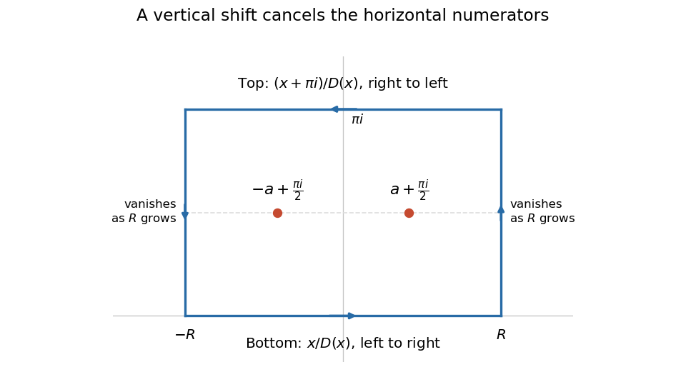
The choice of numerator $z$ makes the horizontal sides useful. The hyperbolic sine satisfies $\sinh (z+\pi i)=-\sinh z$, so $D(x+\pi i)=D(x)$. Consequently the lower and upper contour integrals, with their actual orientations, add toIt remains to justify discarding both vertical sides. On either side $z=\pm R+iy$, $0\le y\le \pi$, the reverse triangle inequality and part (b)(ii) implyThis lower bound is positive for sufficiently large $R$. Also $|z|\le R+\pi$ and each vertical side has length $\pi$. The estimation lemma bounds the absolute value of the sum $V_R$ of the vertical contributions byThe real improper integral converges absolutely, since its integrand is continuous on the real axis and decays like $4e^{-2|x|}$ at infinity. Combining all four sides and taking $R\to \infty$ givesThereforeAn independent real-variable check uses the hyperbolic tangent substitution $u=\tanh x$: the integral becomes ${\int }_{-1}^{1}du/({\cosh }^{2}a-u^2{\sinh }^{2}a)$. Its antiderivative uses the inverse hyperbolic tangent, giving $2\mathrm{arctanh}(\tanh a)/(\sinh a\cosh a)=4a/\sinh (2a)$. As $a\downarrow 0$, this tends to $2$, agreeing with ${\int }_{-\infty }^{\infty }{\mathrm{sech}}^{2}xdx=2$ and checking the factor of two.

Use the principal logarithm $\mathrm{Log}z=\log |z|+i\mathrm{Arg}z$ with $-\pi <\mathrm{Arg}z<\pi$, whose branch cut is the negative real axis. For this choice,has three simple poles away from the cut: $z=1$, $z=ia$, and $z=-ia$. The pole at $1$, caused by $\mathrm{Log}1=0$, must be included.

Choose $0<\epsilon <\min \{1,a\}$ and $R>\max \{1,a\}$, and use a positively oriented keyhole contour around the negative real axis: the large circle is traversed counterclockwise, the upper bank from $-R$ to $-\epsilon$, the small circle clockwise, and the lower bank from $-\epsilon$ to $-R$. Formally, use radial segments at arguments $\pm (\pi -\eta )$, then let $\eta \downarrow 0$ with $R,\epsilon$ fixed. The function has continuous limiting values on each compact bank, which justifies this limit.

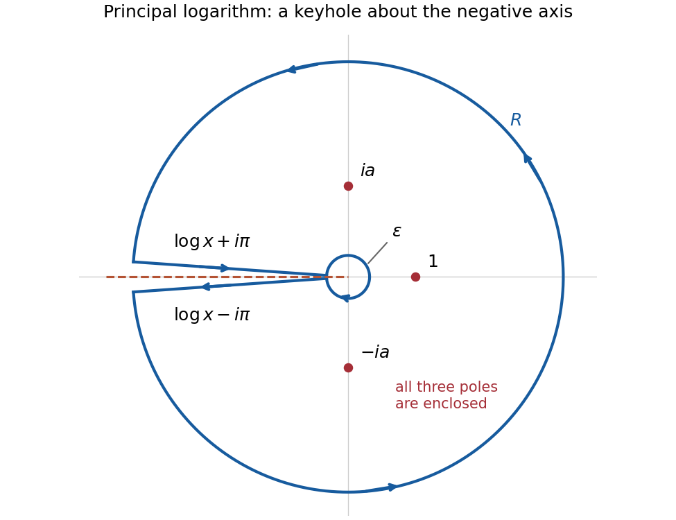
Put $L=\log a$. The residues areThe first follows from $\mathrm{Log}z=(z-1)+O((z-1{)}^2)$; the other two follow from the simple zeros of $z^2+a^2$. Their sum isThese expressions are valid also for $a=1$, since $L\pm i\pi /2$ never vanish for real $L$.

On the outer circle, $|\mathrm{Log}z|\ge \log R$ for $R>1$ and $|z^2+a^2|\ge R^2-a^2$. On the inner circle, $|\mathrm{Log}z|\ge |\log \epsilon |$ and $|z^2+a^2|\ge a^2-{\epsilon }^2$. Thus the estimation lemma bounds the two arc integrals byrespectively, as $R\to \infty$ and $\epsilon \downarrow 0$.

On the upper bank, $z=-x+i0$ gives $\mathrm{Log}z=\log x+i\pi$; on the lower bank it gives $\log x-i\pi$. Accounting for the opposite orientations, their combined integral isThe real improper integral converges: its integrand is bounded near zero by $1/(a^2{\pi }^2)$ and at infinity by $1/({\pi }^2{x}^2)$. Taking the arc limits in the residue theorem gives $-2\pi iI=2\pi i\Sigma$, henceThe final subtraction is exactly the contribution of the pole at $1$.

The improper integral converges: its integrand is bounded near zero and at most $x^{-n}$ for $x\ge 1$, which is integrable because $n\ge 2$.

Set $\theta =\pi /n$, $\omega =e^{2i\theta }$ and $\zeta =e^{i\theta }$. Apply the residue theorem to $F(z)=1/(1+z^n)$ on the positively oriented sector contour consisting of the segment $0\to R$, the arc $R{e}^{it}$ for $0\le t\le 2\theta$, and the segment $R\omega \to 0$, with $R>1$. No pole lies on the boundary. Exactly one root of $z^n=-1$ is inside this sector, namely $\zeta$; it is a simple pole. Part (a) givesOn the returning ray, put $z=\omega x$ with $x$ decreasing from $R$ to zero. Since ${\omega }^n=1$, the two ray contributions areOn the arc, $|1+z^n|\ge R^n-1$, so the estimation lemma bounds its contour integral byThe residue theorem and the convergence already established now giveUsing $1-e^{2i\theta }=-2i{e}^{i\theta }\sin \theta$, we concludeThe sector also works for $n=2$, when it is the upper semicircle. Its angle is chosen so that $z^n$ has the same value on the two rays.

Factor the denominator as $(z^2+1)(z^2+4)$ and integrateover $[-R,R]$ followed by the upper semicircle, for $R>2$. The enclosed simple poles are $i$ and $2i$. The local quotient formula from part (a) givesOn this arc, $|e^{iz}|=e^{-\mathrm{Im}z}\le 1$ and $|z^2+1|\ge R^2-1$, $|z^2+4|\ge R^2-4$. Thus the estimation lemma givesOn the real line, $|F(x)|\le 1/[(x^2+1)(x^2+4)]$, so the improper integral is absolutely convergent. Hence the residue theorem yieldsTaking real parts is justified by absolute convergence. ThereforeThe imaginary part vanishes as a further check, since the sine integrand is odd.