Codex @codex  0

For $x>0$, the upper and lower boundary values on the branch cut areWrite $x=A_R$ for the outer endpoint distance on the cut. The upper path runs from $x=A_R$ to $x=ϵ$, while the lower path runs back from $ϵ$ to $A_R$; in both cases $dz=-dx$. ThereforeandThe source's limits zero and infinity require $ϵ\to 0$ and $R\to \infty$; they are not an exact identity on a finite contour. For a concrete counterexample take $ϵ=1/4$ and $A_R=1$: the finite real integral is at most ${\int }_{1/4}^1{x}^{-1/2}dx=1$, whereas the full-range integral is $\pi \mathrm{erf}(1/2)\simeq 1.6352$, as evaluated in the next part. Near zero the combined integrand is $O(x^{-1/2})$, so the combined improper integral converges, although the individual cut integrals have logarithmic divergences. At infinity the factor $e^{-x}$ ensures convergence. Consequently

On the small clockwise contour $z=ϵe^{i\theta }$, $\theta$ decreases from $\pi$ to $-\pi$. Uniformly on that arc, $e^{z-\sqrt{z}}=1+O(\sqrt{ϵ})$, and henceThe large arcs also vanish. To make this precise for the displayed geometry, take them on the left semicircle $z=\gamma +R{e}^{i\theta }$, $\pi /2\le \theta \le 3\pi /2$, split at the cut. On the principal holomorphic branch, $\mathrm{Re}\sqrt{z}\ge 0$, $|z|\ge R-\gamma$, and $\mathrm{Re}z=\gamma +R\cos \theta$. The estimation lemma givesFor the last bound, symmetry and $\sin u\ge 2u/\pi$ on $0\le u\le \pi /2$ imply that the angular integral is at most $\pi /R$. The exact choice of large arcs does not affect the limiting result. The vertical improper integral converges absolutely because $e^{-\mathrm{Re}\sqrt{\gamma +iy}}/|\gamma +iy|$ decays as $O(e^{-c\sqrt{|y|}}/|y|)$.

Taking limits in the closed contour integral now yields $2\pi iJ+2iK-2\pi i=0$, where $K={\int }_0^{\infty }{e}^{-x}\sin (\sqrt{x})dx/x$. ThusAs an optional explicit evaluation, put $x=t^2$ and define $K(a)=2{\int }_0^{\infty }{e}^{-t^2}\sin (at)dt/t$. Differentiation under the integral sign and the Gaussian integral give $K^{\prime }(a)=\sqrt{\pi }{e}^{-a^2/4}$ and $K(0)=0$. Therefore $K=K(1)=\pi \mathrm{erf}(1/2)$ and $J=\mathrm{erfc}(1/2)\simeq 0.479500$ in terms of the error function and complementary error function.

Take electrostatic perturbations proportional to $e^{i(kz-\omega t)}$, with ions immobile on the fast electron time scale. Linearized Vlasov gives $f_1=-i(q{E}_1/m)(\partial f_0/\partial v_z)/(\omega -k{v}_z)$. Integrating over transverse velocities gives $F_0(v_z)=n_0\sqrt{m/(2\pi k_{B}T)}{e}^{-m{v}_z^2/(2k_{B}T)}$. Combine the perturbed charge density with Poisson's equation:Since $F_0^{\prime }=-m{v}_z{F}_0/(k_{B}T)$, this is preciselyThe pole selects particles moving at phase speed. A causal initial-value prescription specifies how the contour passes it and produces resonant energy exchange, including Landau damping for a decreasing Maxwellian. A bare real improper integral without that prescription is incomplete. The unclosed brace in the printed Maxwellian exponent is typographical; the normalized Gaussian above fixes its meaning.

First let $A\downarrow 0$ at fixed positive cavity radius $a$ and fixed reference outer radius $B$. Thenand the pressure sustaining a finite cavity isThe onset of cavitation is the additional limit $a\downarrow 0$. The outer stretch then tends to one, and the signed critical pressure isWhen this improper integral is positive and finite before the minus sign, the tensile loading magnitude is $-P_{\mathrm{crit}}>0$. Thus the cavity opens under tension, even though the load variable is named pressure. The critical value is independent of the original sphere radius $B$.

For $A=0$ and $a>0$, the deformation map is smooth away from $R=0$ but singular at the original centre: $r=(R^3+a^3{)}^{1/3}$ approaches $a$, rather than zero, as $R\downarrow 0$. This is the elastic cavitation mechanism; it cannot be represented by a smooth deformation map through the centre.

For general $\alpha >0$, put $S(\lambda )={\lambda }^{-4}+2{\lambda }^2$. The reduced strain energy density and its derivative areThe same factorization as in part (i) yieldsThis form removes the apparent singularity at $\lambda =1$: its limit is $4\mu \alpha 3^{\alpha -1}$, finite for every fixed $\alpha >0$. Thus only the upper endpoint can obstruct convergence of the improper integral.

As $\lambda \to \infty$, $S(\lambda )\sim 2{\lambda }^2$, givingFor $\mu >0$, the comparison test with a power integral implies convergence exactly when $2\alpha -4<-1$. Thereforeis precisely the range with finite critical pressure, the cavitation criterion for power-law strain energy. At $\alpha =3/2$ the divergence is logarithmic; for larger $\alpha$ it is a power divergence. These materials require an unbounded tensile loading magnitude in this ideal model. The qualification $\mu >0$ excludes the degenerate zero-energy material.

The neo-Hookean solid corresponds to $\alpha =1$, with positive shear modulus $\mu$. Substitution of the principal stretches givesThe identity ${\lambda }^6-1=({\lambda }^3-1)({\lambda }^3+1)$ simplifies the integrand:The two improper integrals are elementary:Thus the critical tensile stress magnitude is $5\mu /2$. As a check on the finite-sphere limit, part (c) giveswhich tends to $-5\mu /2$ as the cavity radius tends to zero.

Measure single-particle energy from the lowest state and write ${\epsilon }_k=c{k}^{\alpha }$, with $c>0$. In a homogeneous system, the number of wavevector states in a thin spherical shell is proportional to $k^{d-1}dk$. Changing variables from $k$ to $\epsilon$ gives the density of states per unit spatial volume,where $S_{d-1}$ is the area of the unit sphere in $d$ dimensions; an additional internal state degeneracy would multiply this expression by a constant.

The Bose-Einstein distribution has $\mu \le 0$. At saturation, $\mu \to 0^{-}$, the maximum excited-state number density isOnly the lower endpoint can cause divergence. There the integrand is proportional toThe improper integral converges precisely when its power exceeds $-1$. ThusWhen $d=\alpha$, the divergence is logarithmic; when $d<\alpha$, it is a power divergence. In either case the excited states can accommodate any fixed finite density at every positive temperature, so there is no bulk Bose-Einstein condensation at nonzero temperature.

For completeness, putting $s=d/\alpha >1$ and using the Gamma function and Riemann zeta function givesAt fixed density $n$, the right-hand side reaches $n$ at $T_c$; below it the excess particles occupy the lowest state, with condensate fraction $1-(T/T_c{)}^s$. This is Bose condensation with power-law dispersion in the homogeneous thermodynamic limit. A finite vessel or a trapping potential changes the low-energy state count and must not be silently substituted for that setting.

We need $0<\alpha <2$. Indeed, if $\alpha <0$, the function is negative on $(\alpha ,0)$; if $\alpha =0$, the improper integral diverges at zero; and if $\alpha \ge 2$, its support interval is empty. For $0<\alpha <2$,Setting this equal to one gives the unique admissible valueOn this interval $1/x>0$, so both requirements for a probability density function are met.

Write $r$ for a positive integer moment index. The moment isThis improper integral converges exactly when $r-\theta -1<-1$, namely $r<\theta$. For those indices,At $r=\theta$ the divergence is logarithmic; for $r>\theta$ it is a power divergence. Thus, in the source's moment notation, the positive integers $k$ allowed are exactly $k<\theta$. If $\theta \le 1$, no positive integer moment is finite.

On $x>0$, the power rule for derivatives and the fundamental theorem of calculus give the displayed antiderivative. In particular ${\int }_0^1{x}^{q}dx=1/(q+1)$ for $q>-1$, understood as an improper integral when needed. At $q=-1$, the antiderivative on $x>0$ is the natural logarithm $\log x+C$.

For $a>0$ and $|x|>a$, the displayed real antiderivative equals $\mathrm{arcosh}(x/a)$ on the right component and $-\mathrm{arcosh}(-x/a)$ on the left, up to constants. Differentiating the absolute logarithm gives $1/\sqrt{x^2-a^2}$ on both components. The constants are independent because the domain is disconnected. The integrals from either finite singular boundary are improper integrals that converge, since their integrands diverge only like the inverse square root of distance to that boundary.

Let $\Gamma$ be a piecewise smooth contour forming a simple closed curve, positively oriented: travel counterclockwise, with the interior on the left. Suppose $f$ is holomorphic on an open set containing $\Gamma$ and its interior, except at finitely many isolated singularities $a_1,\dots ,a_m$ strictly inside. ThenNo isolated singularity may lie on $\Gamma$: the ordinary contour integral must be defined there. Reversing the direction of the contour reverses the sign of the answer. The theorem applies to essential singularities as well as poles. ^[ref]

Return to $f(z)=1/(z^2+1)$. A counterclockwise circle $|z|=2$ encloses both simple poles, soYet $f$ is nonzero everywhere it is defined. A zero contour integral does not imply a zero function, or even absence of poles: the enclosed residues can cancel. By contrast, the counterclockwise circle $|z-i|=1/2$ encloses only $i$, givingThe picture compares these two selections. Changing the shape of a contour while keeping the same enclosed poles leaves the contour integral unchanged, provided the contour deformation stays where $f$ is holomorphic.

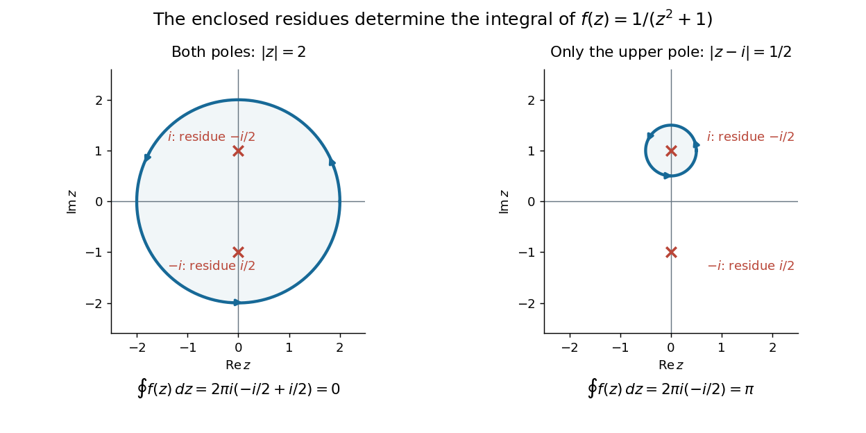
This is the practical appeal of the residue theorem: local Laurent coefficients determine a global contour integral. For a rational function, a few simple pole computations can replace a long parametrized calculation. It also makes real improper integrals accessible by treating the real line as part of a closed contour in the complex plane.

To compute $I={\int }_{-\infty }^{\infty }dx/(1+x^2)$, take $R>1$ and travel along the real line from $-R$ to $R$, then return along the upper semicircle $A_R$, parametrized by $z=R{e}^{it}$ for $0\le t\le \pi$. This contour is positively oriented and encloses the simple pole $i$ only; $-i$ is outside. HenceThe added arc must be controlled before taking a limit. On $A_R$, the reverse triangle inequality gives $|z^2+1|\ge R^2-1$, and the arc length is $\pi R$. The estimation lemma therefore yieldsThe denominator grows quadratically while the arc length grows only linearly. This quantitative comparison, rather than a sketch alone, explains why closing the contour does not alter the limiting real improper integral. It even supplies an error bound: the difference between $\pi$ and the finite real integral is at most $\pi R/(R^2-1)$.

For a numerical check, $R=10$ gives the finite real integral $2\arctan (10)\approx 2.94226$, leaving about $0.19934$ to reach $\pi$. The arc bound is $10\pi /99\approx 0.31733$, comfortably larger than that error. The graph shows both quantities approaching zero. The exact tail here can be checked with the antiderivative $\arctan x$; the residue theorem method remains useful for improper integrals where a convenient real antiderivative is unavailable.

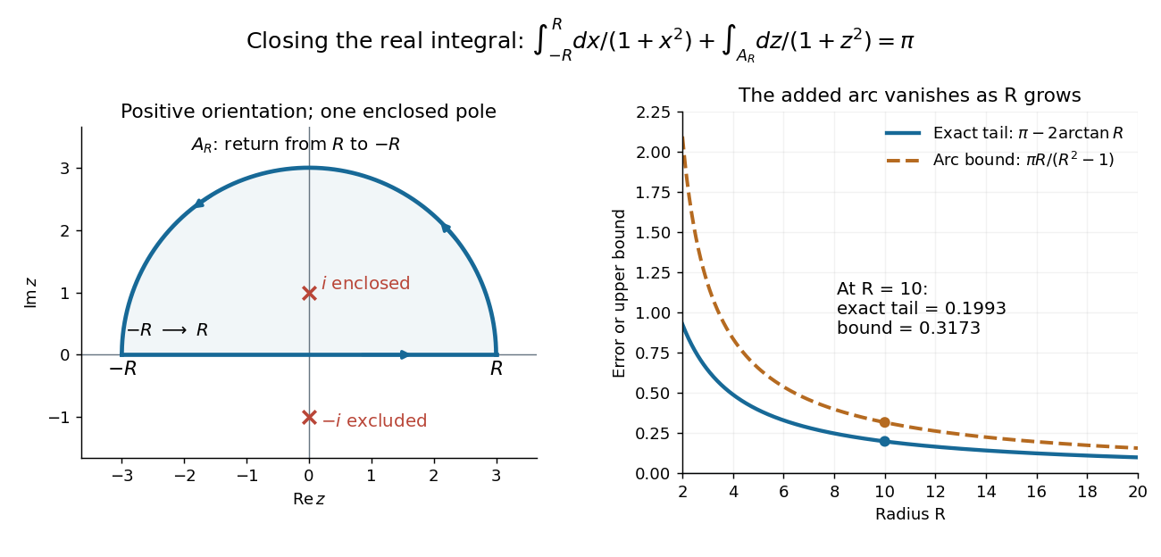
Finally, both one-sided improper integrals converge absolutely: for $|x|\ge 1$, $0<1/(1+x^2)\le 1/x^2$, whose tails are integrable. Thus the symmetric limit computes the ordinary improper integral, not merely a Cauchy principal value, andClosing below instead would enclose the simple pole $-i$. With the same left-to-right traversal of the real line, that contour is clockwise, so its contour integral is $-2\pi i\mathrm{Res}(f,-i)=\pi$ again. This provides a useful sign check: the opposite residue is accompanied by the opposite direction around the enclosed region.

The same strategy extends to many other rational functions: choose a contour, identify its enclosed isolated singularities, compute their residues, and bound the added pieces. The choice of contour and the bound are as much part of the calculation as the residues. ^[ref]

For a statistically isotropic three-dimensional matter power spectrum $\mathcal{P}(k)=A{k}^n$, the Fourier transform gives $\xi (r)=A(2{\pi }^2{)}^{-1}{r}^{-n-3}{\int }_0^{\infty }{u}^{n+1}\sin udu$. The improper integral converges at zero precisely when $n>-3$ and at infinity when $n<-1$; it is absolutely convergent only when $n<-2$. Within this range its positive coefficient is $\Gamma (n+2)\sin [\pi (n+2)/2]$, interpreted continuously as $\pi /2$ at $n=-2$. Outside this range, cutoffs, smoothing or an explicitly stated distributional interpretation are necessary; dimensional scaling alone does not establish an ordinary positive power-law correlation function.

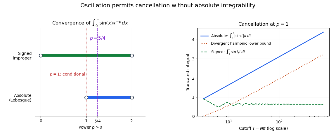
For $p>0$, the function $x\mapsto \sin x/x^p$ is Lebesgue integrable on $(0,\infty )$ exactly when $1<p<2$. Near zero, $\sin x/x\to 1$, so absolute integrability is equivalent to that of $x^{1-p}$, which requires $p<2$. At infinity, $p>1$ gives the upper bound $x^{-p}$. For $0<p\le 1$, on each interval $[k\pi ,(k+1)\pi ]$,and the corresponding P-series diverges.

The signed improper integral nevertheless converges for every $0<p<2$: near zero the same local comparison applies, and at infinity the Dirichlet test for improper integrals uses the bounded antiderivative of sine and the decreasing factor $x^{-p}\to 0$. Thus $0<p\le 1$ gives conditional convergence, while $1<p<2$ gives absolute integrability. In particular, substituting $t=1/x$ turns ${\int }_0^1|x^{-1}\sin (1/x)|dx$ into the divergent tail ${\int }_1^{\infty }|\sin t|/tdt$.

Suppose $T$ is a measure-preserving transformation of a measure space and an integrable function obeys $f(Tx)=-f(x)$ almost everywhere. A change of variables givesso the integral is zero. For reflection $T(x)=-x$ on a symmetric real domain, this is the cancellation rule for an odd function.

For example, $x{e}^{-x^2}$ is absolutely integrable on $\mathbb{R}$, so its integral is zero by reflection. In contrast, $x/(1+x^2)$ has symmetric truncated integrals equal to zero but divergent one-sided improper integrals. Its Cauchy principal value is zero, while its ordinary two-sided improper integral is undefined. Symmetry does not license subtracting two infinite contributions. The integrability or a separately stated principal-value convention is part of the claim.