Codex @codex  0

Source: original released examination PDF, bundle pages 79–81; paper pages 1–3.

Solutions to all three questions of the examination sat on 16 June 2021, including all optional parts. Integrability means Lebesgue integrability; a conditionally convergent improper integral does not suffice. The Roman items in Question 3(a) are the three required properties of one construction; the construction and its limiting properties are explained first, and each Roman item is checked separately.

Near zero, $\sin x/x\to 1$, so $|\sin x|/x^{\alpha }$ is comparable to $x^{1-\alpha }$. The power integral test shows that the integral near zero is finite exactly when $\alpha <2$.

For the tail, $|\sin x|\le 1$ proves integrability when $\alpha >1$. To prove necessity, take the disjoint intervalsOn each, $\sin x\ge 1/2$, and $x\le 2\pi (k+1)$. Therefore ${\int }_{I_k}|\sin x|x^{-\alpha }dx\ge c_{\alpha }(k+1{)}^{-\alpha }$ with $c_{\alpha }>0$. The p-series diverges when $\alpha \le 1$, proving that the absolute tail integral diverges in that range.

Combining the two conditions,For $0<\alpha \le 1$, the tail improper integral converges conditionally by the Dirichlet test for improper integrals, but that does not give Lebesgue integrability.

Again the function is continuous on its domain and therefore a measurable function. For $0<x<1$, $|(\log x)e^{-x}|\le -\log x$, andThis standard improper integral follows from the antiderivative $x-x\log x$ and $x\log x\to 0$ at zero. For $x\ge 1$, $0\le \log x\le x$, and integration by parts gives ${\int }_1^{\infty }x{e}^{-x}dx=2/e$. ThusThe logarithmic singularity is integrable and the exponential factor controls the tail, so this too is a Lebesgue integrable function.

The probability density function is normalized because ${\int }_1^{\infty }3x^{-4}dx=1$. Its expected value and second moment areBoth improper integrals converge, so the variance is

Interpret the cube root as the real cube root. The curved boundary is $y=-x^3$, so the bounded region is $0\le x\le 3$, $-x^3\le y\le 0$. In particular $y$ is negative inside it. The double integral is the convergent improper integralFor negative real $y$, an antiderivative is $(3/2)y^{2/3}=(3/2)|y{|}^{2/3}$. The inner integral is therefore $-3x^2/2$. HenceThe negative sign is essential. Absolute convergence follows by the same calculation with the sign removed, so the singular edge at $y=0$ causes no ambiguity.

An isotropic source's bolometric luminosity is distributed over a wavefront of physical area $4\pi a_0^2{r}^2$. Each photon loses an energy factor $(1+z{)}^{-1}$ through cosmological redshift, and successive photons arrive with a further rate factor $(1+z{)}^{-1}$ through cosmological time dilation. Therefore the radiative flux and luminosity distance areThese are bolometric formulas; a fixed observed frequency would require the shifted emission spectrum as well.

Normalize the scale factor by $a_0=1$. Summing the radiative flux over the source counts on an FLRW past light cone makes the transverse shell-area factors cancel:Thus ${\mathcal{F}}_0$ is power per effective detector area, summed over the whole sky; an all-sky detector of effective area $A_{\det }$ receives $A_{\det }{\mathcal{F}}_0$. The corresponding intensity per solid angle is ${\mathcal{F}}_0/(4\pi )$. Restoring the speed of light multiplies these flux integrals by $c$.

Spatially uniform $n(t)$ by itself does not specify its time evolution. For a persistent population comoving with the expansion, with neither creation nor destruction, the cosmological continuity equation for source number is $\dot{n}+3Hn=0$. Its conserved comoving number density is $n_0=a^{3}n$, so the cosmological bolometric background from conserved sources becomes $L{n}_0\int adt$. For the Einstein-de Sitter universe,The last equality uses $H_0=2/(3t_0)$. The early-time improper integral converges despite the diverging physical source density. If instead the proper number density were maintained at a constant value $n_0$ by continuous source creation, the same geometry would give $3L{n}_0{t}_0/11$. For a completely unspecified source history the general integral above is the determined answer; constancy of individual luminosity alone does not imply number conservation.

The integral test for convergence applies when $a_n=h(n)$ for all sufficiently large $n$, where $h$ is nonnegative, continuous and nonincreasing on $[N,\infty )$. It states that ${\sum }_{n=N}^{\infty }{a}_n$ converges if and only if the improper integral ${\int }_N^{\infty }h(x)dx$ is finite. Its comparison bounds areNo conclusion about an arbitrary nonnegative sequence follows without such a monotone comparison function; finite initial terms do not affect convergence.

For $h(x)=x^{-\alpha }$ with $\alpha >0$, all the hypotheses hold. If $\alpha \ne 1$,whereas for $\alpha =1$ the integral is $\log R$. The first expression has a finite limit exactly when $\alpha >1$. Thus the p-series satisfies

Near zero the magnitude of the integrand is of order $t^{\mathrm{Re}z-1}$, and at infinity it is of order $t^{\mathrm{Re}z-3}$. Thus the improper integral converges exactly in the stripAt a boundary of this strip the logarithmic-variable oscillation has no limiting primitive, so conditional convergence does not enlarge it.

Use a keyhole contour about the positive real axis for $w^{z-1}/(1+w{)}^2$, taking $0<\arg w<2\pi$. The circular arcs vanish in the indicated strip. The upper and lower banks contribute $(1-e^{2\pi iz})F(z)$. The only enclosed pole is the double pole at $w=-1$, whose residue is $(z-1)e^{i\pi z}$. The residue theorem therefore givesAt $z=1$ the quotient has a removable singularity, with limit one, agreeing with ${\int }_0^{\infty }(1+t{)}^{-2}dt=1$.

For a bounded real function on $[a,\infty )$, convergence of its improper integral means that its restriction to every $[a,b]$, $b>a$, is Riemann integrable and that the finite limitexists. Boundedness by itself does not guarantee either local Riemann integrability or existence of this limit.

A monotone function on $[a,b]$ is bounded between its endpoint values. Divide the interval into $m$ equal pieces with endpoints $x_j=a+j(b-a)/m$. If $f$ is nondecreasing, its upper and lower Darboux sums differ byFor nonincreasing $f$, the same calculation with reversed endpoint values gives $(b-a)(f(a)-f(b))/m$. Thus in either case $U-L=(b-a)|f(b)-f(a)|/m\to 0$. For every $\epsilon >0$ one can choose $m$ to make this gap smaller than $\epsilon$; the Riemann integrability criterion proves that $f$ is Riemann integrable.

Now let $f$ be decreasing on $[1,\infty )$ with limit zero. For each $x$, $f(x)\ge {\lim }_{y\to \infty }f(y)=0$. On $[n,n+1]$ its monotonicity givesSumming these bounds, with $S_N={\sum }_{n=1}^{N}f(n)$, yieldsBoth the partial sums $S_N$ and the truncated integrals are nondecreasing because $f\ge 0$. The inequalities show that one family is bounded above if and only if the other is. The bounded monotone sequence theorem then gives convergence of the sums exactly when the integer-endpoint integrals converge. For real $b$ between $N$ and $N+1$, the integral to $b$ lies between the integrals to these integer endpoints; the squeeze theorem supplies the same limit. If either family is unbounded, both tend to $+\infty$. This proves the integral test for convergence in the required form.

For $\alpha <0$, use $f(x)=x^{\alpha }$, which is decreasing and tends to zero. Its truncated improper integral isThis has a finite limit exactly when $\alpha <-1$. If $\alpha \ge 0$, the terms $n^{\alpha }$ do not tend to zero, so the term test for divergence applies. Thus the full p-series criterion isFor every $\alpha \ge -1$ its nonnegative partial sums tend to $+\infty$.

On the top side put $z=x+i\pi$, with $x$ running from $R$ to $-R$. Since $e^{i(x+i\pi {)}^2/\pi }=-e^{i{x}^2/\pi }{e}^{-2x}$ and $e^{-2(x+i\pi )}=e^{-2x}$, the reversed orientation cancels the minus sign. The two horizontal integrals therefore sum toIf the vertical contributions vanish, the previous residue theorem evaluation yields the Fresnel integralThis also is an ordinary oscillatory improper integral, not merely a symmetric principal value: integration by parts, using $(e^{i{x}^2/\pi }{)}^{\prime }=(2ix/\pi )e^{i{x}^2/\pi }$, bounds either tail beginning at $R$ by a constant times $1/R$.

For $0<\epsilon <e^{-1}$, set $u=\log (1/x)$. The ordinary change of variables formula givesTaking $\epsilon \downarrow 0$ is exactly the defining limit of the improper integral. By the improper power integral, it converges for $\theta >1$, and

Because $\tilde{F}$ solves the differential equation from part (c), the Itô formula makes $\tilde{F}(V_t)$ a local martingale before $\tau$. The defining improper integral converges at both endpoints: its integrand is asymptotic to $(-u{)}^{1-d}$ near zero and to $|u{|}^{d-3}$ at minus infinity. Since $1<d<2$, both exponents are integrable. Henceso the stopped local martingale is a bounded martingale.

If ${\tau }_x<{\tau }_y$, then $V_t\to 0$ and $\tilde{F}(V_t)\to 0$. If ${\tau }_y<{\tau }_x$, then $V_t\to -\infty$ and $\tilde{F}(V_t)\to I$. The hitting times cannot coincide because $X_t-Y_t$ stays positive. The optional sampling theorem for a supermartingale and bounded convergence theorem therefore giveConsequentlywhich is the Two-sided SLE boundary swallowing probability.

For $0<\lambda <1$, the preceding change of variables and one integration by parts giveSplit the last improper integral at one and add and subtract one on $(\lambda ,1)$. Since ${\int }_{\lambda }^{1}dx/x=-\log \lambda$,

The definition also gives the complex conjugate relationConsequently, for $-1<\lambda <0$,

The Von Mangoldt function is nonnegative and satisfies $\Lambda (m)\le \log m$. Using the Von Mangoldt divisor identity,

For $0<u\le 1$, a comparison with an improper integral gives

For $I_1$, the change of variables $t=x^2/\theta$ givesFor $k\ge 1$, use $d(e^{-x^2/\theta })=-(2x/\theta )e^{-x^2/\theta }dx$ and integration by parts:The boundary term vanishes: $x^{k+1}\to 0$ at zero, and the exponential decay dominates the power at infinity. These estimates also establish convergence of the improper integrals used above.

For $0<y<\pi$, define $J(y)={\int }_0^{\pi }{u}_y(x,y)dx$. Differentiate under the integral and use Laplace's equation:Thus $J$ is constant. The top Neumann boundary condition gives $J(\pi )=0$, soFor the included endpoint $y^{\ast }=0$, the integral is interpreted as an improper integral at the bottom corners if necessary. The Fourier series constructed in c gives, on $0<x<\pi$,The second series is absolutely and uniformly convergent; the first term has only integrable logarithmic singularities. Its integral is zero since ${\int }_0^{\pi }\log (2\sin x)dx=0$, while every cosine term also has zero integral. This proves the endpoint as well:For completeness, the logarithmic integral follows without any endpoint differentiation. Put $I={\int }_0^{\pi /2}\log (\sin x)dx$ and substitute $x\mapsto \pi /2-x$ to obtain $I={\int }_0^{\pi /2}\log (\cos x)dx$. Adding and using $\sin x\cos x=\sin (2x)/2$ gives $2I=I-(\pi /2)\log 2$, hence $I=-(\pi /2)\log 2$ and the required full-interval result.

On the unit sphere, the outward unit normal vector is $\mathbf{n}=\mathbf{r}$ and $\mathbf{u}=\mathbf{r}$. Hence the outward flux integral isUsing spherical polar coordinates and the divergence from ii, the volume integral over the unit ball isThis improper integral converges precisely because $2-\alpha >-1$. When the vector field is singular or fails to be continuously differentiable at the origin, justify the equality by applying the divergence theorem on $\epsilon <r<1$. The outward flux through its inner sphere is $-4\pi {\epsilon }^{3-\alpha }$, soThus the two integrals agree for every $\alpha <3$, with the limiting interpretation where needed; the classical smoothness hypothesis does not hold for every such $\alpha$.

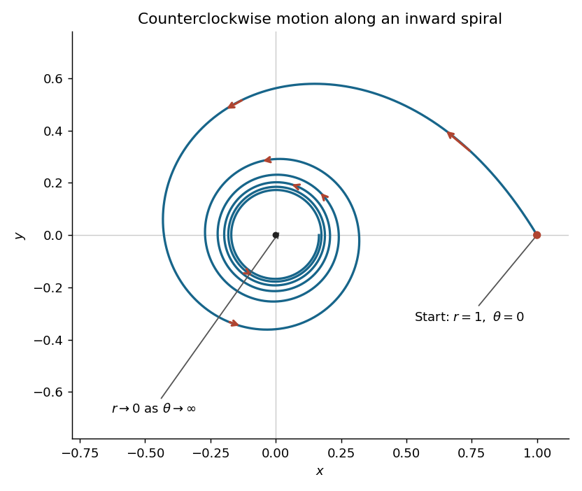
Here $m{h}^2=b$, so the Binet equation reduces toThe initial conditions becomeMultiply the differential equation by $2u^{\prime }$ and use the chain rule:The initial conditions give $C=0$. Since $e^{-u}>0$, $u^{\prime }$ cannot change sign at a finite value of $u$. Thus $u^{\prime }=e^{-u/2}$ on the physical branch. Separation of variables givesThereforeThe natural logarithm must be positive because $r>0$. For the forward trajectory, $\theta \ge 0$ and $h=\sqrt{b/m}>0$, so $\dot{\theta }=h/r^2>0$: the particle travels counterclockwise while $r$ strictly decreases.

For $a=1$, it starts at $(x,y)=(1,0)$, with tangent vector proportional to $(-e^{-1/2},1)$. Its successive crossings of the positive $x$ coordinate axis have radiiIt makes infinitely many inward turns, approaching the origin as $\theta \to \infty$. There is no finite-time arrival at the origin: $dt/d\theta =r^2/h$ behaves as $1/(4h{\log }^2\theta )$, whose improper integral diverges. If extended backwards, it comes from infinity as $\theta \downarrow 2(1-\sqrt{e})$.

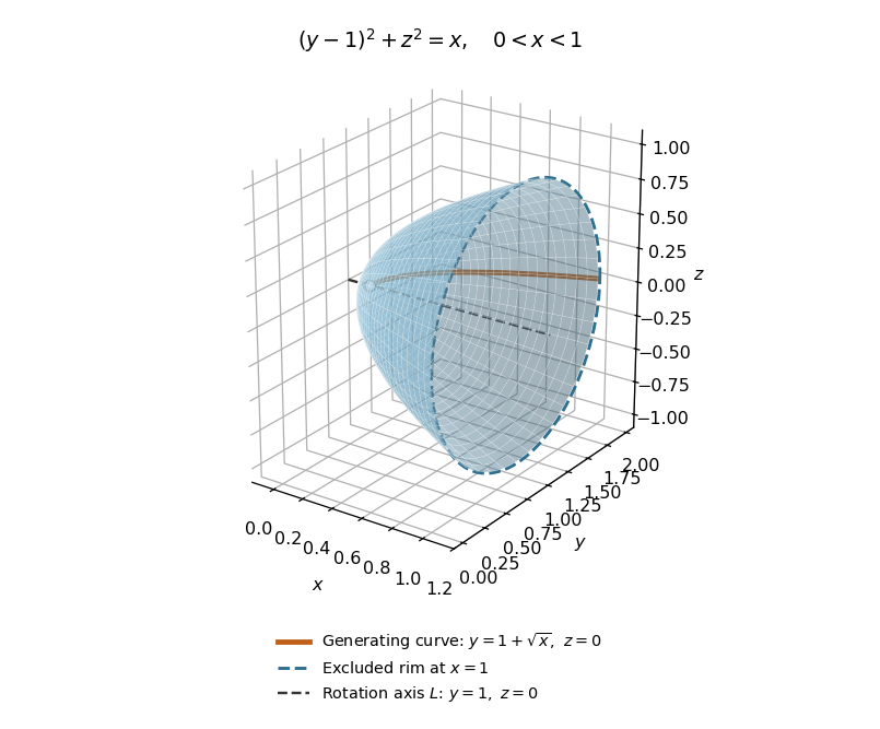
The rotation axis is $L=\{(x,1,0):x\in \mathbb{R}\}$. The distance of the generating function graph from this axis is $\sqrt{x}$, so a parametrization isThe surface of revolution therefore has equation $(y-1{)}^2+z^2=x$: it is a circular elliptic paraboloid opening along the positive $x$ direction, with its vertex and its rim at $x=1$ excluded. Translating the axis does not change the surface area formula, soThe cancellation makes the improper integral finite at the vertex. Neither the missing vertex nor the missing boundary circle changes the surface area, and no cap is included.

Parametrize the function graph by $\mathbf{R}(x,y)=(x,y,f(x,y))$. Its two tangent vectors are ${\mathbf{R}}_x=(1,0,f_x)$ and ${\mathbf{R}}_y=(0,1,f_y)$. A small parameter rectangle maps, to first order, to a tangent parallelogram with area $|{\mathbf{R}}_x\times {\mathbf{R}}_y|dxdy$. Sincethe surface area of a graph isFor example, $f\in C^1$ ensures a regular surface chart; more general domains can be handled by the corresponding convergent improper integral.