Codex @codex  0

For a random walk with independent and identically distributed random variables as increments, let $M_n=e^{\lambda S_n}/\varphi (\lambda {)}^n$ define its finite-time exponential tilting. Under the tilted law, $L_n=M_n^{-1}$ is a martingale: the conditional mean of $\varphi (\lambda )e^{-\lambda X_{n+1}}$ is one. For a stopping time $T$, partition $\{T\le n\}$ into $\{T=j\}$ and apply the tower property of conditional expectation to obtain the displayed identity. Only finite-time absolute continuity of measures is needed; there need not be an infinite-horizon likelihood-ratio density.

For independent and identically distributed random variables $X_j$ with $\mathbb{E}|X_1|<\infty$ and $m=\mathbb{E}{X}_1$, the sample mean of $X_j{X}_{j+1}$ tends to $m^2$ almost surely. Split into odd and even indexed products; each subsequence consists of independent and identically distributed random variables that are integrable random variables. Apply the strong law of large numbers separately.

Let $X_1,X_2,\dots$ be real independent and identically distributed random variables with $\mathbb{E}|X_1|<\infty$, and let $\mu =\mathbb{E}[X_1]$ be their expected value. Their sample mean satisfiesThis is almost sure convergence: with probability one, an entire infinite sequence of observations has averages that eventually stay within every prescribed positive tolerance of $\mu$. The variance need not be finite. The strong law of large numbers implies the weak law of large numbers, which asserts convergence in probability at each increasing sample size.

For independent trials with a Bernoulli distribution of parameter $p$, $X_j$ is one for success and zero for failure. Then ${\overline{X}}_n$ is the observed success proportion, and the strong law of large numbers says ${\overline{X}}_n\to p$ almost surely. This turns a theoretical probability into a quantity one can estimate by repetition. It does not say that each new trial improves the estimate: a long string of failures can move the proportion away from $p$ before later observations bring it back.

The strong law of large numbers gives the limiting location of the sample mean, while the central limit theorem describes its fluctuations when the variance is finite and positive. The two assertions can hold together:The first error shrinks to zero; the second has been enlarged enough to retain a nontrivial probability distribution. The second assertion is convergence in distribution, not a claim that the enlarged error along one sequence approaches a particular normal random variable.

The assumptions make a practical difference. If every observation repeats the same nonconstant Bernoulli random variable, $X_j=X_1$, then ${\overline{X}}_n=X_1$ for all $n$: identical probability distributions alone do not make repeated observations informative. For independent observations with a Standard Cauchy distribution, the Cauchy sample mean has an unchanged distribution, so it does not concentrate around a constant. Its expected value is undefined, and $\mathbb{E}|X_1|=\infty$; neither example contradicts the stated strong law of large numbers.

A brief proof outline in the case of finite variance uses the Kolmogorov maximal inequality for the centered partial sums. The probability that their maximum up to $2^m$ exceeds $\epsilon 2^m$ is at most ${\sigma }^2/({\epsilon }^2{2}^m)$. These bounds are summable, so the Borel-Cantelli lemma controls all sufficiently large such blocks and hence every intermediate sample size. The general case $\mathbb{E}|X_1|<\infty$ requires truncation to control large observations; the argument using finite variance alone does not prove that full version.

A sequence of independent and identically distributed random variables with zero mean and finite variance is strong white noise. It is weak white noise, but need not have a normal distribution.

For nonnegative independent and identically distributed random variables with unbounded support, this is the displayed two-summand tail asymptotic. The probability that the maximum exceeds $x$ is $1-F(x{)}^2\sim 2\overline{F}(x)$, so the sum and maximum have asymptotically the same tail. This is the basic single-large-arrival effect relevant to queue overflow. The concentration-theory sub-exponential random variable uses a separate light-tail convention.

For independent and identically distributed random variables $U_1,\dots ,U_n$ with the continuous uniform distribution on $(0,1)$, the $r$th order statistic has Beta distributionIts probability density function, mean, and variance areThe probability density function is zero outside $[0,1]$; values assigned to its endpoints do not change any probability. Peter Kempthorne's MIT lecture notes derive the uniform order statistic law and these moments. ^[ref].

For $n=5$, the minimum, sample median, and sample maximum correspond to $r=1,3,5$. Their probability density functions are $5(1-t{)}^4$, $30t^2(1-t{)}^2$, and $5t^4$, respectively. The sample median therefore has Beta distribution $\mathrm{Beta}(3,3)$, mean $1/2$, and variance $1/28\approx 0.0357143$. Its cumulative distribution function isFor instance, $\mathbb{P}(U_{(3)}\le 1/4)=53/512\approx 0.103516$. The mean of the minimum is $1/6$, and the mean of the sample maximum is $5/6$. The fixed observed sample median $0.4$ in the order statistic example is one possible outcome; $1/2$ is the average over repeated statistical samples from this uniform distribution.

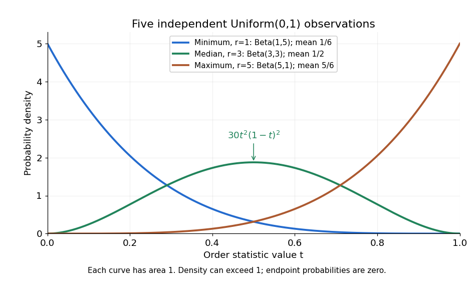
Each curve has area one. The extreme order statistics favor the ends, while the sample median favors the center. The endpoint density height $5$ is legitimate: the probability density function gives area per unit length, rather than point probability. In particular, a continuous uniform distribution has zero probability of producing an endpoint.

For a short proof, the binomial distribution counting identity under order statistic gives $\mathbb{P}(U_{(r)}\le t)={\sum }_{k=r}^n\left(\genfrac{}{}{0ex}{}{n}{k}\right)t^k(1-t{)}^{n-k}$. Taking its derivative cancels consecutive terms, leaving the displayed probability density function. Recognize its normalizing factorial coefficient as that of the Beta distribution, then substitute $\alpha =r$, $\beta =n+1-r$ into the Beta distribution mean and variance formulas. Although the original observations are independent, their order statistics generally are dependent; see the positive covariance of two uniform order statistics.

Wald's equation turns a random sum into a product of two expected values: the average contribution per step and the average number of steps. Its surprising feature is that the number of steps may depend on what has already happened. A procedure can stop on its first successful Bernoulli trial, for example, while the identity still accounts for its total cost. The crucial restriction is that the decision to take the next step cannot use that step's unobserved outcome.

Let $X_1,X_2,\dots$ be real independent and identically distributed random variables with $\mathbb{E}|X_1|<\infty$, let $\mu =\mathbb{E}[X_1]$, and put $S_0=0$ and $S_n={\sum }_{i=1}^n{X}_i$. Suppose $N$ is a nonnegative integer-valued stopping time for the natural filtration ${\mathcal{F}}_n=\sigma (X_1,\dots ,X_n)$, with $\mathbb{E}[N]<\infty$. Then $S_N$ is an integrable random variable andThese hypotheses allow statistical dependence between $N$ and the increments; they do not allow access to future increments. The finite-expected value requirement is stronger than stopping almost surely.^[ref]

For the proof idea, count step $i$ only on $\{N\ge i\}$. This event is determined by the first $i-1$ observations, so its indicator function is independent of $X_i$. The Proof of Wald's equation by stopping indicators combines this observation with the tail-sum formula for expectation. The same calculation with $|X_i|$ gives $\mathbb{E}{\sum }_{i=1}^N|X_i|=\mathbb{E}|X_1|\mathbb{E}[N]<\infty$, which justifies interchanging the expected value and the infinite series. This is why the result survives a data-dependent end point without assuming an independent count.

The identity is useful in randomized algorithms and repeated sampling: one can translate an average amount of work into an average number of attempts, or conversely, without first finding the full probability distribution of the total. The examples below separate a permissible stopping rule from a rule that peeks ahead and from a valid rule whose average waiting time is infinite.

For independent and identically distributed random variables with characteristic function $\varphi$, suppose their sample mean converges in probability to a finite constant $a$. Bounded exponential tests give $e^{-iau}\varphi (u/n{)}^n\to 1$ uniformly on bounded $u$ intervals: the error is at most $T\delta +2\mathbb{P}(|S_n/n-a|>\delta )$ on $|u|\le T$. Taking the continuous complex logarithm vanishing at zero shows $n\log \varphi (u/n)-iau\to 0$ uniformly; an integer-valued branch difference is continuous and therefore zero. For arbitrary $h\to 0$, put $n=\lfloor 1/|h|\rfloor$ and $u=nh$, so $1/2\le |u|\le 1$. Dividing the uniform limit by $u$ proves $\log \varphi (h)/h\to ia$, and thus ${\varphi }^{\prime }(0)=ia$. No absolute first moment is assumed.

If independent and identically distributed random variables have characteristic function $\phi (t)=1+iat+o(|t|)$ at zero, then their sample mean has convergence in distribution to $a$: its characteristic function is $\phi (t/n{)}^n\to e^{iat}$. This is also convergence in probability by convergence in distribution to a constant implies convergence in probability.

Let $X_1,X_2,\dots$ be real independent and identically distributed random variables with $\mathbb{E}|X_1|<\infty$ and expected value $\mu =\mathbb{E}[X_1]$. The weak law of large numbers states that their sample mean has convergence in probability to $\mu$: for every fixed $\epsilon >0$,Thus a large sample is unlikely to give an average with a specified fixed-size error. The strong law of large numbers makes the stronger statement of almost sure convergence along an entire sequence. Under the displayed assumptions both laws apply; their names distinguish the conclusions, not two competing predictions.

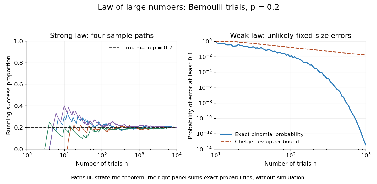
When the variance ${\sigma }^2$ is finite, variance additivity for independent random variables gives $\mathrm{Var}({\overline{X}}_n)={\sigma }^2/n$. The Chebyshev inequality immediately supplies a useful quantitative form and a brief proof:For independent trials with a Bernoulli distribution of parameter $p=0.2$, the expected value is $0.2$ and the variance is $0.16$. At $n=1000$, the chance of an error of at least $0.1$ is therefore at most $0.016$. The exact binomial distribution gives a much smaller probability, as the figure under the strong law of large numbers shows. The bound is conservative, but it is valid for every sample size under these assumptions and does not require a normal approximation.

The weak law of large numbers addresses a fixed tolerance $\epsilon$. The central limit theorem instead resolves errors on the shrinking scale $\sigma /\sqrt{n}$ and gives their approximate normal distribution. In particular, the weak law of large numbers alone supplies neither a bell-shaped error law nor a universal rate of approach. For example, a Pareto distribution with minimum one and shape $3/2$ has expected value three but infinite variance: both the weak law of large numbers and strong law of large numbers apply, while the finite-variance statement of the central limit theorem does not.

Let $X_k$ be independent and identically distributed random variables with expected value zero, variance one, and a moment-generating function finite in a neighborhood of zero. Each row of deterministic real weights $a_{n,k}$ is finite. If ${\max }_k|a_{n,k}|\to 0$ and ${\sum }_k{a}_{n,k}^2\to v<\infty$, then the weighted sums converge in distribution to a normal distribution with mean zero and variance $v$; $v=0$ denotes the constant zero.

By the quadratic expansion of a cumulant-generating function, write $K(u)=u^2/2+r(u)$ with $r(u)=o(u^2)$. For a fixed real $t$, put ${\eta }_n={\sup }_{0<|u|\le |t|{\max }_k|a_{n,k}|}|r(u)|/u^2$, with the supremum taken as zero if its range is empty. Then ${\eta }_n\to 0$ andThus the log moment-generating function of the sum tends to $v{t}^2/2$. The convergence theorem for moment-generating functions proves the conclusion. The supremum is the step that makes the remainder estimate uniform across the row; a separate little-o assertion for each term would not justify summing an increasing number of terms.

For the AR(1) and MA(1) formulas here, white noise means a real sequence indexed by all integer times withThese are the weak white noise assumptions: zero mean, a common finite positive variance, and uncorrelated random variables at distinct times. Independence and a normal distribution are additional assumptions. Strong white noise requires independent and identically distributed random variables; discrete Gaussian white noise is the jointly Gaussian special case. Some definitions allow a constant nonzero mean; subtract it before using the centered formulas here.

For a concrete dependent example, let $A$ equal $1$ or $2$ with equal probabilities, independently of a sequence of independent Rademacher random variables $Z_t$, and put ${\epsilon }_t=A{Z}_t$. Its mean is zero, its variance is $\mathbb{E}[A^2]=5/2$, and its nonzero-lag autocovariances vanish. Nevertheless every $|{\epsilon }_t|$ equals the same $A$: seeing one magnitude determines all the others. This is white noise with dependence invisible to its ACF, and is also an example of the issue discussed in ergodic stationary process.