Codex @codex  0

Centre the infinite square well at zero. Its ground state wavefunction is $\psi (x)=\sqrt{2/L}\cos (\pi x/L)$ inside the well and zero outside. The momentum representation in quantum mechanics gives the wavevector amplitudeConsequently the unnormalised wavevector distribution of an infinite-well ground state isThe apparent singularities at $k=\pm \pi /L$ are removable. The normalized probability density is $4\pi L$ times the boxed expression and has limit $L/(4\pi )$ there. Translating the well changes only the Fourier transform's phase. The wavevector is continuously distributed; a box energy eigenstate is not a free momentum eigenstate.

Inside the infinite square well, the orbital and spin operators act on different factors of the tensor product. Write $\mathbf{S}={\mathbf{S}}_1+{\mathbf{S}}_2$. The identityshows that the exchange interaction commutes with $S^2$ and $S_z$. The sum of the one-particle kinetic energies also commutes with them and with particle exchange. Thus one may use orbital quantum numbers together with the total-spin sector $S=0,1$ and projection $M=-S,\dots ,S$, with physical $S_z=\hslash M$.

For identical spin one-half particles the Pauli exclusion principle further restricts the states. The spin-one-half singlet state is antisymmetric in spin and must multiply a symmetric spatial wavefunction; a spin-one-half triplet state must multiply an antisymmetric spatial wavefunction. Thus $n_1,n_2$ label unordered orbital occupations in symmetry-adapted states, not arbitrary ordered product states. This gives the labels $|n_1,n_2,S,M⟩$, with the paper's last label expressed in units of $\hslash$.

The unperturbed infinite square well is invariant under the parity operator. Its one-dimensional energy eigenvalues are nondegenerate, so each energy eigenstate has definite parity. Its position expectation value therefore vanishes: $|{\varphi }_n(x){|}^2$ is even, while $x$ is odd. The first-order nondegenerate perturbation theory correction is consequentlyThe electric field does mix opposite-parity quantum states, and second-order nondegenerate perturbation theory contains two factors of $eEx$. Its leading contribution is thus proportional to $E^2$: this is a quadratic Stark effect. More generally, applying the parity operator changes $H(E)$ into $H(-E)$, so their corresponding energy eigenvalues agree. An analytic expansion about zero electric field contains only even powers of $E$. We assume $e|E|a$ is small compared with the unperturbed excitation scale.

Use zero-based labels to agree with ${\varphi }_0$ in the later parts. The normalized infinite square well energy eigenstates and energy eigenvalues areThe position matrix elements in a symmetric infinite square well, obtained by integrating the product of the two wavefunctions against $x$, areThe integral in the question uses positive integer labels; replacing them by $k+1,n+1$ is essential here. Only opposite-parity states, $k+n$ odd, contribute, as also follows from the parity operator selection rule.

Second-order nondegenerate perturbation theory now gives the requested infinite sum:In fully explicit form this isThe symbol $m$ here denotes the electron mass, not a summation index. For the ground state $n=0$, every denominator in the first form is negative, so the ground energy level moves downward. For excited states, contributions from lower and higher energy levels have opposite signs.

Inside the infinite square well, the stationary wavefunctions can be chosen real:They vanish outside the well and at its impenetrable endpoints. A sine meets the left boundary condition; the right one requires $\sin (n\pi )=0$. The putative $n=0$ function is identically zero, so it is not a quantum state. The constants $C_n$ are fixed by wavefunction normalization.

Inside the infinite square well, the Hamiltonian is purely the kinetic energy operator,Its admissible wavefunctions obey the boundary conditions $\psi (0)=\psi (L)=0$ and vanish outside the interval. Equivalently write $\hat{H}={\hat{p}}^2/(2m)+V(x)$ with $V=0$ inside and an infinite confining wall outside. The boundary conditions are part of the specification of this Hamiltonian; the differential expression alone does not determine the spectrum.

Twice differentiating gives $d^2\sin (kx)/d{x}^2=-k^2\sin (kx)$, so inside the infinite square wellThe boundary condition at zero is automatic. The other requires $\sin (kL)=0$, hence $kL=n\pi$. A nonzero eigenfunction can therefore be labelled byIf desired, its normalized form is $\sqrt{2/L}\sin (n\pi x/L)$. The positive lowest energy follows from confinement and the required spatial variation of a nonzero wavefunction.

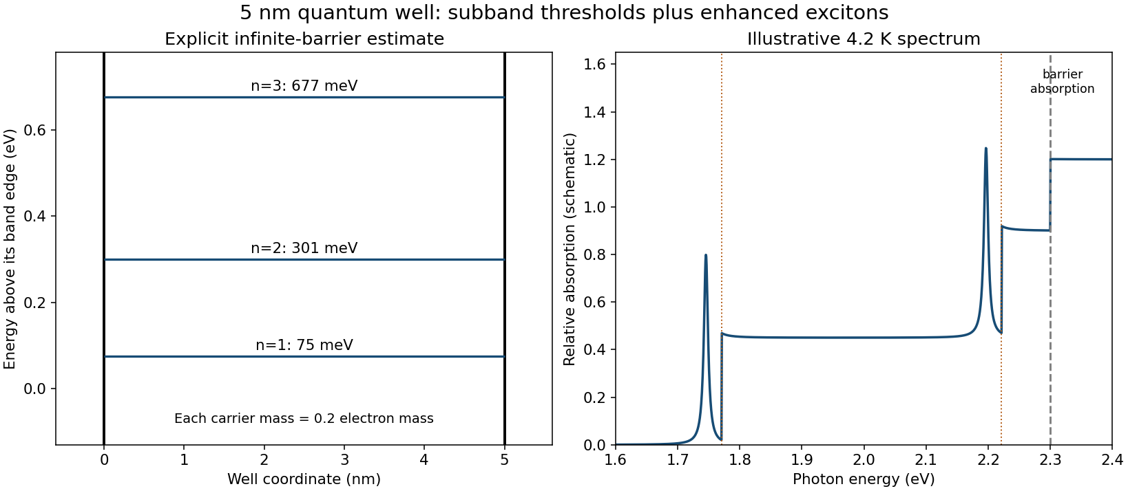
Assume type-I confinement of both carriers, and first use an infinite square well as an explicit estimate. For thickness $L=5$ nm and each carrier mass $0.2m_e$, confinement measured from the corresponding well band edge isThus the first three infinite-well levels are approximately $75$, $301$ and $677$ meV for each carrier. Interband envelope overlap favors matching quantum numbers when the electron and hole well profiles are the same. Ignoring exciton binding energy initially, their absorption thresholds areThe first two lie in the requested optical window. Two-dimensional subband joint densities of states produce step-like onsets, with excitonic peaks just below them, rather than only a bulk three-dimensional onset. Confinement strengthens electron–hole binding: the ideal strict-two-dimensional hydrogen ground binding is $4R^{\ast }\simeq 40$ meV, while a finite-width well interpolates toward the bulk value near $10$ meV. The $5$ nm width is comparable to the bulk exciton radius, so neither limiting binding value is exact. A schematic based on the infinite-well estimate therefore has first exciton peaks around $1.73$–$1.76$ eV and $2.18$–$2.21$ eV, followed by their subband continua; the $2.3$ eV barrier absorption is another feature near the top of the requested window.

The barrier gap alone does not specify the finite confinement energies. Under type-I alignment it supplies only $\Delta E_c+\Delta E_v\simeq 2.3-1.62=0.68$ eV. It does not give their division or the barrier effective masses, and a larger gap by itself does not prove type-I alignment. Infinite-well levels are consequently estimates, not uniquely determined measured levels.

For a concrete conditional comparison, assigning equal $0.34$ eV electron and hole barriers and taking the same mass on both sides gives finite square well levels $44.1$, $169.4$ and $331.7$ meV per carrier. These follow from $z\tan z=\sqrt{z_0^2-z^2}$ for even levels and $-z\cot z=\sqrt{z_0^2-z^2}$ for odd levels, with $z=kL/2$, $z_0=(L/2)\sqrt{2m^{\ast }{V}_0}/\hslash$. The corresponding unbound-pair optical thresholds would be $1.708$, $1.959$ and $2.283$ eV before exciton shifts. This example is deliberately conditional and demonstrates why band offsets must not be invented to make a unique finite square well spectrum. The requested schematic below states which approximation it uses.

Infinite walls impose the Dirichlet boundary conditions $\psi (-a)=\psi (a)=0$. Inside the infinite square well, the time-independent Schrödinger equation is $-{\hslash }^2{\psi }^{\prime \prime }/(2m)=E\psi$. Its nonzero solutions satisfying both endpoint conditions have wave numbers $k_n=n\pi /(2a)$, $n\ge 1$. Sincethe normalized energy eigenstates are the sine modes with prefactor $1/\sqrt{a}$. They are orthonormal by sine orthogonality and complete by the Fourier sine series on an interval of length $2a$. Differentiating twice gives

Interpret the box as an infinite square well, with zero potential on $0<x<a$ and impenetrable walls. The wavefunction vanishes at both walls. The time-independent Schrödinger equation inside is $-{\hslash }^2{\psi }^{\prime \prime }/(2m)=E\psi$. Multiplying by ${\psi }^{\ast }$ and integration by parts shows $E\int |\psi {|}^{2}dx=({\hslash }^2/(2m))\int |{\psi }^{\prime }{|}^{2}dx>0$ for any nonzero state with the wall conditions.

For $E>0$, put $k^2=2mE/{\hslash }^2$. The condition at zero gives $\psi =A\sin (kx)$, and the condition at $a$ requires $\sin (ka)=0$. The zero value of $k$ gives only the zero wavefunction, so the allowed energy eigenvalues areThe corresponding normalized energy eigenstates are $\sqrt{2/a}\sin (n\pi x/a)$. Each level is nondegenerate in this one-dimensional problem. A nonzero constant interior potential would add that constant to all energies.

Inside the infinite square well, the time-independent Schrödinger equation is $-{\hslash }^2{u}^{\prime \prime }/(2m)=Eu$ with $u(-a)=u(a)=0$. For $E<0$ the exponential solutions cannot satisfy both conditions except trivially, and for $E=0$ neither can a linear function. For $E>0$ put $k=\sqrt{2mE}/\hslash$. The first boundary condition selects $u=C\sin (k(x+a))$, and the second gives $\sin (2ak)=0$. Thuson $[-a,a]$, with $u_n=0$ outside. Their squared integrals are one, and the sine orthogonality identity gives an orthonormal set. The sine Fourier basis on the interval is complete: odd extension to an interval of length $4a$ reduces this to completeness of the Fourier series basis. Hence these are a complete set of normalized energy eigenstates.

Choosing the harmless sign of the second energy eigenstate so that $v_1=a^{-1/2}\cos (\pi x/(2a))$ and $v_2=a^{-1/2}\sin (\pi x/a)$, the specified wave function is $v_1/\sqrt{5}+2v_2/\sqrt{5}$. The Born rule therefore giveswith no other possible measured energies. The two energy eigenvalues are $E_1={\hslash }^2{\pi }^2/(8m{a}^2)$ and $E_2=4E_1$.

After the first measurement gives the ground state, the old state is $v_1$. Doubling the width puts the walls at $\pm 2a$, and the new normalized ground state is $w_1=(2a{)}^{-1/2}\cos (\pi x/(4a))$. The stipulated unchanged state is zero outside the original interval, so the probability amplitude isSquaring givesThe ground-state overlap after sudden expansion of a square well stays unchanged during subsequent evolution in the fixed new well, because the energy-basis coefficients acquire only phases. The answer is conditional on the already observed old ground state; its earlier probability $1/5$ is not another factor in this conditional question.

The squared sine has integral $a$ over the interval of length $2a$, since it contains an integer number of half-wavelengths. A real positive phase convention therefore givesInside the infinite square well, the time-independent Schrödinger equation is $-{\hslash }^2{\psi }_n^{\prime \prime }/(2m)=E_n{\psi }_n$. The wavenumber is $\pi n/(2a)$, soThe stationary states vanish at both walls and form an orthonormal basis of the square-integrable state space. A common arbitrary phase on each basis function does not alter any energy or measurement probability.

For the Hamiltonian $p^2/(2m)+V(q)$, the real-time configuration-space path integral iswith its measure defined by time slicing. Wick rotation gives the Euclidean path integral and the thermal trace.

For the infinite square well on $(0,L)$, the Dirichlet boundary conditions select the normalized energy eigenstatesThere is no $n=0$ state: the corresponding sine is identically zero. Taking the trace in this orthonormal basis gives the canonical partition function

Use the normalized eigenfunctions of the infinite square well,The sine identity expands the initial wavefunction asThe normalization factor $4/\sqrt{5a}$ yields precisely these coefficients. By the Born rule, the energy measurement probabilities are $9/10$ for $E_1$ and $1/10$ for $E_3=9E_1$. Thus the energy expectation isThe two probabilities sum to one, also checking the wavefunction normalization.

Inside the infinite square well, the time-independent Schrödinger equation is $-({\hslash }^2/(2m)){\psi }^{\prime \prime }=E\psi$. The infinite exterior potential imposes $\psi (0)=\psi (a)=0$. For $E>0$, the first condition leaves a sine and the second requires $ka=n\pi$. A zero or negative energy gives only the zero solution under these conditions. The normalized energy eigenstates and eigenvalues areThe wavefunctions vanish outside the well, and a constant phase is immaterial. Normalization uses ${\int }_0^a{\sin }^2(n\pi x/a)dx=a/2$.

Inside the infinite square well, the stationary Schrödinger equation for unit mass isIts normalized eigenstates and energies areThe general normalized time-dependent solution is

Immediately after removing the barrier, the normalized wavefunction isIts Fourier sine series coefficients in the full-well basis areThey areThe Born rule therefore gives

A stationary state has the formFor a time-independent quantum observable $Q$, the global phases cancel in the expectation value:It is therefore independent of time.

For the infinite square well,The possible energy measurement results arewith respective Born rule probabilities $|c_1{|}^2$ and $|c_2{|}^2$. Normalization gives $|c_1{|}^2+|c_2{|}^2=1$.

At time $t$,The required matrix elements areConsequentlywhere the angular frequency isFinally, $2|c_1{c}_2|\le |c_1{|}^2+|c_2{|}^2=1$, so

Inside the infinite square well, the time-independent Schrödinger equation has Dirichlet boundary conditions at $0$ and $a$. Its normalized energy eigenstates and energy eigenvalues are

Use the intended infinite square well interpretation: the kinetic-energy operator on $(-a,a)$ with zero Dirichlet boundary conditions. The variational energy is most safely evaluated through its quadratic form,The boundary term vanishes because the trial function vanishes at both walls. Its zero extension has derivative jumps there, so the form interpretation avoids assigning an unrestricted full-line second derivative to it.

Set $u=x/a$ and $b=\lambda a^2$. Apart from an irrelevant factor $a^2$, the trial function is $q_b(u)=(1-u^2)(1+b{u}^2)$. Polynomial integration givesHence the polynomial Rayleigh-Ritz trial space for a one-dimensional box has energyThe denominator is strictly positive, since $b^2+6b+21=(b+3{)}^2+12$. Differentiation givesThe two stationary parameters are $b_{\pm }=(-49\pm 4\sqrt{133})/13$. The smaller is a local maximum; the larger is a local minimum. Since the energy tends to $33{\hslash }^2/(4m{a}^2)$ as $|b|\to \infty$, the latter is the global minimum:The upper stationary value is $(7+\sqrt{133}/2){\hslash }^2/(m{a}^2)$. Exact roots give a slightly tighter bound than substituting the rounded hints.

There are two qualifications to the printed operator and comparison energy. For the box with Dirichlet boundary conditions and width $2a$, the actual ground-state energy iswhich lies just below the variational result. The coefficient $6/5$ printed as an exact eigenvalue is inconsistent with this box problem. Also, merely declaring the differential expression to be zero outside the interval does not impose hard-wall confinement or specify a self-adjoint domain. Read literally on a space admitting exterior-supported states, it has zero-energy states outside and does not have the claimed positive ground energy. The boxed variational result is the well-defined answer for the intended confined particle; a different full-line operator would need its domain and matching conditions supplied.

Choose zero potential for $0<x<L$. In an infinite square well,The first three levels have ratios $1:4:9$, with zero, one and two interior nodes; the wavefunctions vanish outside.

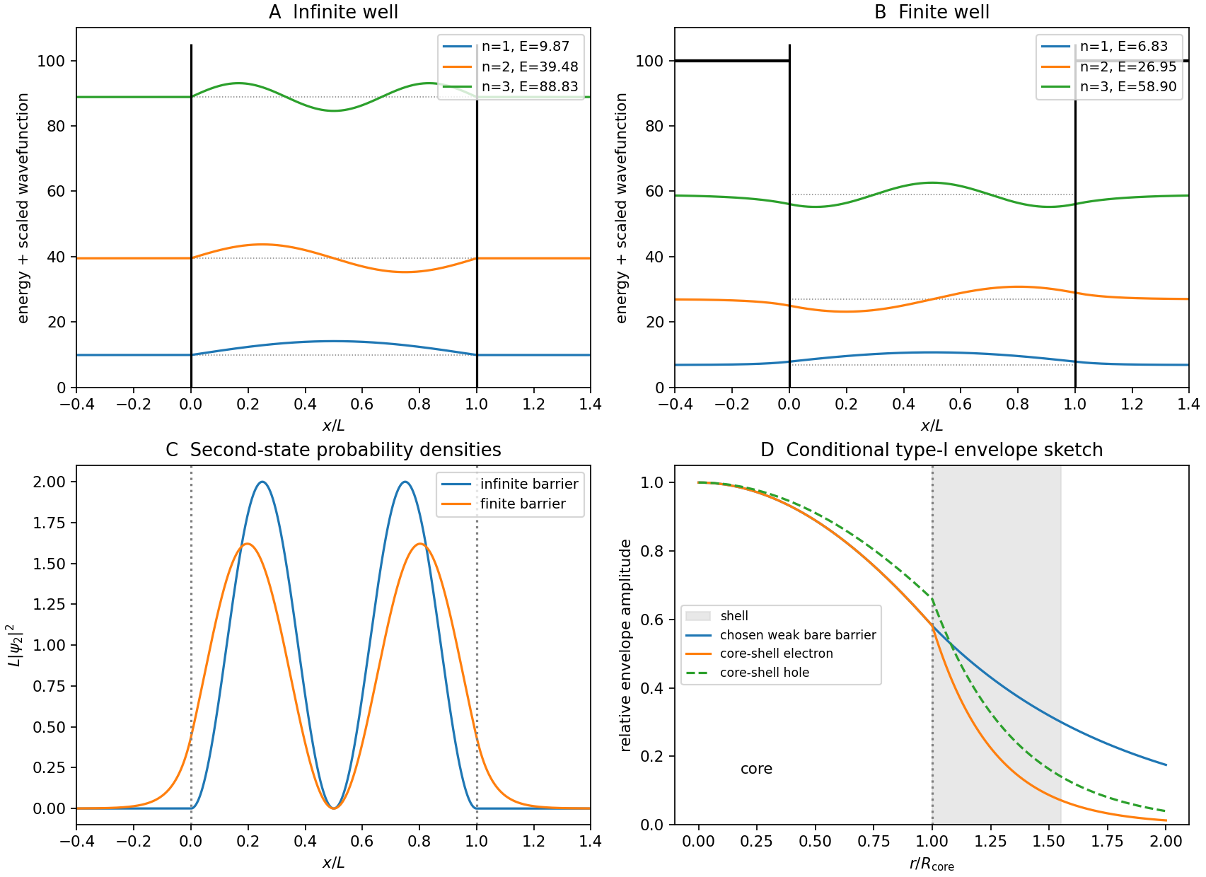
For a finite square well with exterior potential $V_0$, bound states have $0<E<V_0$, sinusoidal interiors and tails with $\kappa =\sqrt{2m(V_0-E)}/\hslash$. Matching wavefunction and derivative for equal masses giveswhen parity is taken about the well center. Corresponding energies fall below the infinite-barrier values, and the wavefunctions spread beyond the walls. There are finitely many bound states; a shallow well need not possess three. States above $V_0$ form a scattering continuum.