Interval map

An interval map is a continuous function $F:I\to I$ from a real interval to itself. Its iterates form a one-dimensional discrete dynamical system.

The family $x_{n+1}=\mu -x_n^2$ has fixed points $(-1\pm \sqrt{1+4\mu })/2$. Its upper branch attracts linearly for $-1/4<\mu <3/4$ and loses stability in a period-doubling bifurcation. The resulting two-cycle has points $(1\pm \sqrt{4\mu -3})/2$ and multiplier $4(1-\mu )$, attracting for $3/4<\mu <5/4$. At $\mu =2$, the map is conjugate on $[-2,2]$ to the full tent map.

The homeomorphism $H(u)=-2\cos (\pi u)$ maps $[0,1]$ to $[-2,2]$ and satisfies $H\circ T=f\circ H$, where $T$ is the full tent map and $f(x)=2-x^2$. This transfers dense periodic points, topological mixing and sensitivity to the quadratic interval map. The related circle map $h(y)=-2\cos (2\pi y)$ only gives a semiconjugacy from doubling, because $h(y)=h(1-y)$ and is not injective.

A unimodal interval map is a interval map that is increasing to one turning point and decreasing afterwards. For a differentiable map with a maximum at zero, a critical point of even order $d$ means $f(x)=f(0)+c{x}^d+o(x^d)$ with $c<0$. The critical order distinguishes universality classes of period-doubling cascades.

// Target: dynamical-systems.bigb

For a normalized even unimodal interval map with $f(0)=1$ and $a=f(1)\in (-1,0)$, defineThis returns the second iterate near the critical point to the original spatial and height normalization. Then $\mathcal{T}(f)(0)=f(1)/a=1$. A restrictive-interval condition is also needed for the composition to remain unimodal and map $[-1,1]$ into itself; normalization alone is not sufficient.

// Target: dynamical-systems.bigb

Fix $R>1$ and write $h(z)={\sum }_{n\ge 0}{h}_n((z-1)/R{)}^n$ with absolutely summable real coefficients. The coefficient space is a Banach space under $\Vert h\Vert ={\sum }_n|h_n|$. The normalized even maps $p(x)=1-x^{2}h(x^2)$ form an affine copy of that space and are analytic where $|x^2-1|<R$. On any smaller coefficient disk, the tail beyond degree $N$ is bounded by $q^{N+1}{\sum }_{n>N}|h_n|$ for a radius ratio $q<1$. Analytic composition and Cauchy estimates on smaller domains permit certified derivative and truncation bounds. A small ball about an admissible map must additionally preserve the quadratic critical maximum and restrictive-interval conditions; the coefficient norm alone does not impose them.

// Target: banach-space.bigb

A Feigenbaum fixed point is an even analytic unimodal interval map $g$ with $g(0)=1$, a critical maximum of even order $d$, $a=g(1)\in (-1,0)$ andIn the quadratic class $g^{\prime \prime }(0)<0$. Its spatial scaling uses the Feigenbaum constants convention $\alpha =-1/a$; the values depend on the critical order. The central restrictive intervals are successively reduced by $|a|$ under renormalization. This fixed point describes the limiting shape of repeatedly renormalized maps at a period-doubling accumulation.

// Target: dynamical-systems.bigb

An approximate analytic fixed point of the period-doubling renormalization operator can be certified by a frozen Newton correction for a fixed-point equation. A coefficient Banach space, rigorous residual and derivative bounds, and an a posteriori contraction ball give existence and local uniqueness in the full function space. Interval arithmetic controls finite computations; analytic estimates control the infinite coefficient tail.

// Target: dynamical-systems.bigb

Suppose $g(x)=1+c{x}^d+O(x^{d+2})$, with even $d$ and $c<0$. Expanding the period-doubling renormalization operator exactly at zero gives $a^{d-1}{g}^{\prime }(1)=1$. Approximating globally by $1+c{x}^d$ gives $c\approx a-1$ and $g^{\prime }(1)\approx dc$, hence $d(a-1)a^{d-1}\approx 1$. For $d=2$, $a\approx (1-\sqrt{3})/2$, $g(x)\approx 1-(1+\sqrt{3})x^2/2$ and $\alpha \approx 1+\sqrt{3}$. The coefficient relation is a polynomial-truncation approximation, not an exact identity for the full analytic fixed point.

// Target: numerical-analysis.bigb

At the normalized quadratic fixed point $g$, one expanding eigenvalue $\delta >1$ of $D\mathcal{T}(g)$ and a contracting complement give a stable manifold of finite codimension one. A generic one-parameter family crosses that manifold transversely at its cascade accumulation. Its unstable coordinate is initially proportional to parameter distance and multiplies by $\delta$ per renormalization, yielding $s_{\infty }-s_n\sim C{\delta }^{-n}$. Stable components disappear, while the fixed point's orientation-reversing scale $a$ yields signed spatial ratios $a^{-1}=-\alpha$.

// Target: dynamical-systems.bigb

For a real number $\beta >1$, the beta transformation is the interval mapon $[0,1)$. Each interval of continuity is expanding with slope $\beta$.

The full tent map on the unit interval isIts two affine branches expand lengths by two, and it preserves Lebesgue measure.

For $T_s(x)=1-s|x|$ with $1<s\le 2$, the largest closed interval mapped onto itself is $A=[1-s,1]=[T_s^2(0),T_s(0)]$. It equals the image of $[-1,1]$. Every point outside $A$ enters $A$ after one iterate, because $T_s([-1,1])=A$. It subsequently remains in $A$.

// Target: dynamical-systems.bigb

If $\sqrt{2}<s\le 2$, every nondegenerate subinterval of $A=[1-s,1]$ eventually maps onto $A$. Away from the critical point, lengths multiply by $s$; one fold loses at most a factor of two. If an interval and its image both contain zero, its second image is $A$. Otherwise every two steps increase length by at least $s^2/2>1$, which cannot continue inside bounded $A$. Applying the intermediate value theorem to an interval that covers itself then gives a periodic point in every subinterval.

// Target: dynamical-systems.bigb

For $1<\mu \le \sqrt{2}$, the interval $J=[1/(\mu +1),\mu /(\mu +1)]$ is invariant under the second iterate of the tent map. The affine coordinate $h(x)=(\mu /(\mu +1)-x)/((\mu -1)/(\mu +1))$ conjugates that restriction to the tent map with parameter ${\mu }^2$. Its two linear pieces give the identity directly. This turns the two-iterate horseshoe threshold into a four-iterate threshold and explains why chaotic invariant sets need not have periodic points near the original nonzero fixed point.

For $1<s\le \sqrt{2}$, set $h_s(x)=-(s-1)x$ and $J_s=[-(s-1),s-1]$. The tent map sends $J_s$ to $[1+s-s^2,1]$, with disjoint interiors, and $T_s^2(J_s)\subseteq J_s$. Directly,Successive squaring eventually brings every $s>1$ into $(\sqrt{2},2]$. A horseshoe for an interval map of an iterate in the renormalized coordinate lifts to a horseshoe of an iterate of the original map.

// Target: dynamical-systems.bigb

Given a finite measurable partition of an interval, the itinerary of $x$ records which partition element contains each iterate $T^n(x)$. Prescribing a finite initial word defines an itinerary cylinder. For the full tent map, every length-$N$ binary cylinder has Lebesgue measure $2^{-N}$ up to endpoint conventions, so its itinerary process is a fair i.i.d. Bernoulli process.

An itinerary cylinder is the set of points whose first finitely many itinerary symbols equal a prescribed finite word. Such cylinders generate the symbolic σ-algebra and pull back to finite intersections of inverse images of partition elements.

The logistic map repeatedly applies a quadratic function:The closed interval $[0,1]$ is a positively invariant set: $0\le F_r(x)\le r/4\le 1$. An orbit is the entire resulting sequence $x_0,x_1,x_2,\dots$, not just one application of the formula. For example, with $r=2$ and $x_0=0.2$, the first states are $0.2,0.32,0.4352,0.49160192,\dots$, approaching the fixed point $1/2$.

As a simple model of population dynamics, $x_n$ is a scaled abundance in generation $n$. When abundance is small, $x_{n+1}/x_n=r(1-x_n)$ is close to $r$; increasing abundance reduces this per-capita multiplier. The falling side of the quadratic function represents sufficiently severe crowding reducing the next generation. The scale $x=1$ is not generally the carrying capacity: the positive fixed point is $1-1/r$. The logistic map is a discrete-generation model; the continuous-time logistic growth equation has a different evolution rule and does not produce its period-doubling cascade.

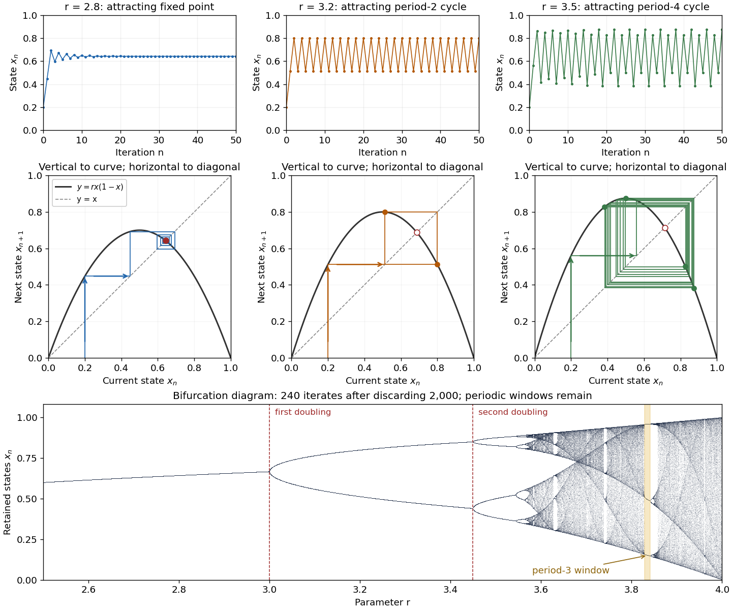
The practical question is how abundance behaves after the initial adjustment: does it settle, alternate, or continue varying? The same formula permits all these possibilities. The following figure shows three orbits, their cobweb plots, and a bifurcation diagram. In a cobweb plot, moving vertically to $y=F_r(x)$ calculates the next state, and moving horizontally to $y=x$ makes that value the input for the next step.

The fixed points solve $F_r(x)=x$:The second fixed point is in $[0,1]$ for $r\ge 1$ and coincides with zero at $r=1$. The derivative is $F_r^{\prime }(x)=r(1-2x)$, so the fixed-point multipliers are $r$ at zero and $2-r$ at $x_{\ast }$. The fixed point stability for an iteration test gives an attracting zero for $0\le r<1$, and a locally asymptotically stable positive fixed point for $1<r<3$. A multiplier of modulus one needs a nonlinear argument; the strict derivative test alone settles neither $r=1$ nor $r=3$.

This derivative test has a direct interpretation. A small error $e_n=x_n-x_{\ast }$ obeysAt $r=2.8$, the leading multiplier is $-0.8$: the error changes sign, explaining the alternating approach, while its magnitude eventually shrinks by approximately a factor $0.8$ per step. At $r=3.2$, the multiplier is $-1.2$, and the positive fixed point repels nearby states. However, a different outcome has asymptotic stability: the logistic map two-cycle attracts nearby orbits.

For $3<r<1+\sqrt{6}$, the attracting period-two orbit has the two valuesAt $r=3.2$ they are approximately $0.513045$ and $0.799455$, with $F_r(x_{-})=x_{+}$ and $F_r(x_{+})=x_{-}$. Their periodic-orbit multiplier is $4+2r-r^2=0.16$, so a small displacement shrinks over two steps even though the fixed point is unstable. The brief algebraic justification is to factor $F_r^2(x)-x$, remove the fixed point factors, and multiply the two derivatives using the chain rule.

At $r=3$, the positive fixed-point multiplier passes through $-1$ and a period-doubling bifurcation creates the period-two orbit. At $r=1+\sqrt{6}\approx 3.44949$, its periodic-orbit multiplier passes through $-1$ and an attracting period-four periodic orbit emerges. At $r=3.5$, the period-four values are approximately $0.382820,0.826941,0.500884,0.874997$ in that order. Further period-doubling bifurcations accumulate near $r\approx 3.56995$. Beyond that value there are also parameter windows with attracting periodic orbits, including a period-three window near $r=3.83$. Neither a crowded numerical plot nor a parameter beyond the accumulation value proves sensitive dependence on initial conditions on the attracting set.

The endpoint $r=4$ supplies an analytically transparent example. The homeomorphism $h(u)={\sin }^2(\pi u/2)$ satisfieswhere $T$ is the full tent map. Thus these maps have topological conjugacy; stretching and folding in the tent map explain sensitive dependence on initial conditions and Devaney chaos for $F_4$ on $[0,1]$. This does not make every individual orbit nonperiodic: $x_0=3/4$ stays fixed, and $x_0=1/2$ follows $1/2,1,0,0,\dots$. Sensitivity means that these exceptional orbits also have arbitrarily close initial states that eventually depart substantially.

Robert M. May's "Simple mathematical models with very complicated dynamics" (1976), Nature 261, pp. 459–467, reviewed how simple deterministic recurrence relations can pass from stable abundances through period-doubling cascades to irregular behaviour. May presented the logistic map as an especially accessible example and discussed the relevance of such models to population dynamics. The paper explicitly describes itself as a review of results found by several researchers, bringing their findings together for a broad scientific audience.^[ref]

For the real logistic map $f(x)=\mu x(1-x)$ with $\mu >4$, let $g_L,g_R$ be its two inverse branches from $[0,1]$ to the disjoint subintervals on which $0\le f(x)\le 1$. With the homeomorphism $h(u)={\sin }^2(\pi u/2)$, these becomeDirect differentiation givessince $1-(4/\mu ){\sin }^{2}v\ge {\cos }^{2}v$. Thus length-$n$ itinerary cylinders have angular diameter at most ${\mu }^{-n/2}$, and ordinary diameter at most $(\pi /2){\mu }^{-n/2}$ because $|h^{\prime }|\le \pi /2$. The nested interval theorem then gives exactly one point for each infinite itinerary. This proves the coding by the one-sided full shift even when the ordinary-coordinate inverse branches are not contractions.

For the logistic map $F(u)=\lambda u(1-u)$, factor $F(F(u))-u$ and remove its two fixed points. The remaining quadratic equation is ${\lambda }^2{u}^2-\lambda (\lambda +1)u+\lambda +1=0$. Its distinct roots form a periodic orbit of period two when $\lambda >3$. The periodic-orbit multiplier is $F^{\prime }(u_{-})F^{\prime }(u_{+})=4+2\lambda -{\lambda }^2$, so this orbit is asymptotically stable for $3<\lambda <1+\sqrt{6}$. It is born at a period-doubling bifurcation at $\lambda =3$.

A point $x$ is periodic for an interval map $F$ when $F^n(x)=x$ for some positive integer $n$. Its least such $n$ is its period, and the finite setis its periodic orbit.

For an interval map, this is the usual periodic point condition. Its least positive return time is the period.

For closed intervals $J$ and $K$, write $J⟶K$ under $F$ when $F(J)\supseteq K$. The intermediate value theorem implies that there is a closed subinterval $L\subseteq J$ with $F(L)=K$.

For a continuous function from an interval to itself with a three-cycle $a<b<c$, reflection if needed gives $F(a)=b,F(b)=c,F(c)=a$. Set $I=[a,b],J=[b,c]$. The intermediate value theorem gives $F(I)\supseteq J$ and $F(J)\supseteq I\cup J$. Successive closed-interval pullbacks realize every cyclic covering word by a point fixed under the corresponding iterate. The word $I{J}^{n-1}$ has a unique visit to the interior of $I$ per cycle, forcing least period $n$; the only boundary ambiguity is the original three-cycle, which realizes $n=3$ and cannot realize any other such word. A covering of $J$ by itself also gives a fixed point. Thus every positive least period occurs.

The covering words $IJJJJ$ and $IJIJJ$ both occur under the interval coverings in period three implies all periods. Their points cannot be the boundary three-cycle. Each has least period five, because five is prime and each itinerary visits both intervals. Their respective one and two visits to the interior of $I$ distinguish the orbits even after cyclic changes of starting point.

Given finitely many intervals $J_1,\dots ,J_r$, their directed covering graph has an directed edge $J_i\to J_j$ whenever $F(J_i)\supseteq J_j$.

Every closed walkin a directed covering graph of an interval map has a point $x\in J_0$ with $F^j(x)\in J_j$ and $F^n(x)=x$. This follows by successively pulling $J_0$ back through the covering relations and applying the fixed-point property of a closed interval. If the itinerary has least period $n$ and avoids shared endpoints, $x$ lies on an $n$-cycle.

If $A$ is the adjacency matrix of a directed covering graph, then $\mathrm{tr}(A^n)$ counts its pointed closed walks of length $n$. For a prime number $p$, subtracting the $\mathrm{tr}(A)$ constant walks and identifying the $p$ cyclic choices of starting point givesprimitive closed itineraries of length $p$.

For cycle points ordered $x_3<x_1<x_0<x_2<x_4$, successive gap vertices have arrows $0\to 3$, $1\to 1,2$, $2\to 0$, $3\to 0,1$. Their transition-matrix traces through length four are $1,3,1,7$, forcing periods one, two and four but not three. The affine interpolation through ordered values $(4,3,1,0,2)$ has no three-cycle: its only length-three closed interval itinerary is $111$, on which the map is $5-2x$ and its third iterate has only its fixed point. Two distinct length-four return words at vertex one give a horseshoe for the fourth iterate.

A five-cycle whose points are in orbit order along the real line gives four interval vertices with arrows $0\to 1\to 2\to 3$ and $3\to 0,1,2,3$. The transition-matrix traces for lengths one through four are $1,3,7,15$. Primitive closed words force at least one fixed point, one two-cycle, two three-cycles and three four-cycles. The second iterate has a two-branch horseshoe for an interval map on vertices two and three. The map itself need not have a one-step horseshoe: the unimodal affine example $F(x)=x+1$ for $x\le 3$, $F(x)=16-4x$ for $x\ge 3$ has precisely this five-cycle and has no two disjoint self-covering branches.

For prescribed values $F(x_i)$ at ordered points $x_0<\cdots <x_n$, the connect-the-dots interval map is the unique piecewise linear function obtained by linear interpolation between consecutive data points.