Codex @codex  0

A real positive-semidefinite kernel satisfies $|k(x,y){|}^2\le k(x,x)k(y,y)$. This follows from positivity of its two-point kernel matrix. If a diagonal value is zero, the corresponding off-diagonal values must also vanish.

For $d$ input coordinates, the homogeneous quadratic polynomial kernel has a weighted quadratic feature map with $D=d(d+1)/2$ distinct monomials. Computing an inner product of already stored mapped vectors costs $O(D)$ arithmetic operations, whereas $(x^{T}z{)}^2$ costs $O(d)$ using the input vectors. Here $O$ denotes big O notation. Higher fixed degrees can make the dimension gap much larger.

Sample count still matters. With $n$ training examples, materializing a dense kernel matrix stores $n^2$ numbers and requires $n(n+1)/2$ distinct evaluations using symmetry. A dense direct solve for kernel ridge regression typically takes $O(n^3)$ operations after constructing the kernel matrix, while a dual prediction with $m$ nonzero coefficients uses $m$ kernel evaluations. Explicit finite feature maps can be preferable when $D$ is small relative to $n$, and a stored primal weight vector can make prediction depend on $D$ rather than on $n$. The kernel trick by Ryan Giordano (sections Ridge regression and The polynomial kernel) explains the change from feature-coordinate equations to training-example equations; neither representation is universally faster.

The kernel trick saves explicit feature construction when the positive-semidefinite kernel is economical to evaluate; it does not remove the cost of optimization, choose a useful positive-semidefinite kernel, or establish generalization. Random Fourier features illustrate a different tradeoff: replacing the exact Gaussian kernel with a finite approximate feature map can reduce dependence on the sample count while introducing approximation error.

If the weight vector lies in the linear span of the training feature map outputs, write $w={\sum }_i{\beta }_i\varphi (p_i)$. ThenThis is a dual representation: coefficients weight training examples rather than feature coordinates. They need not be positive, and need not be unique when the kernel matrix is singular. 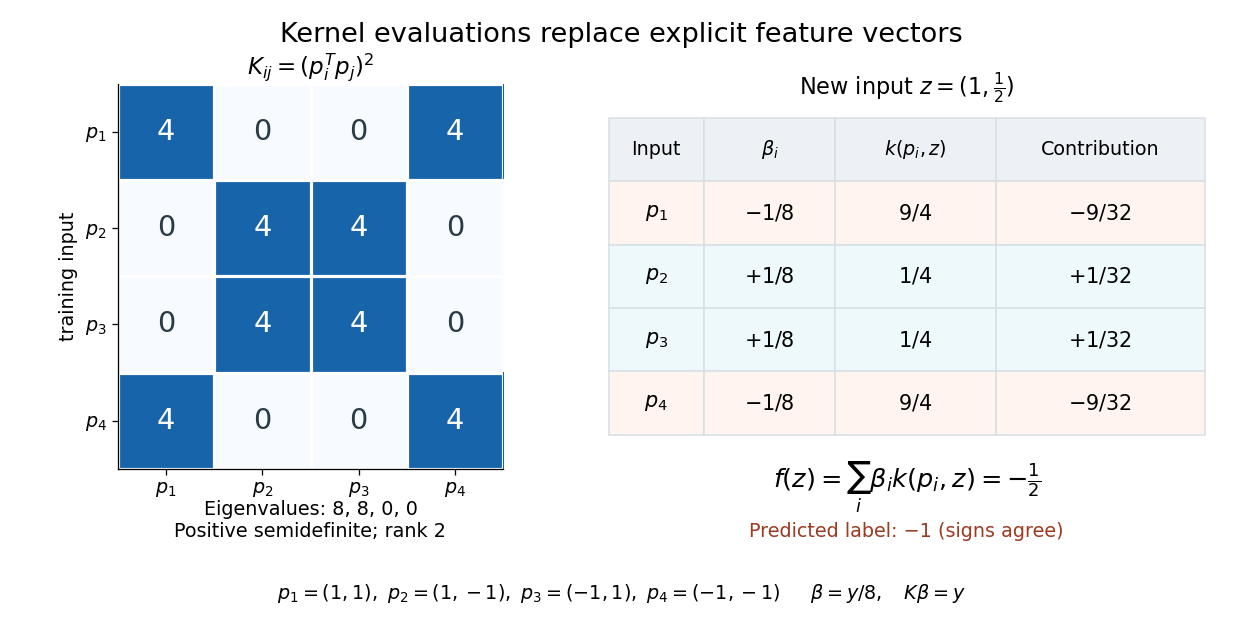Some kernel methods instead write ${\beta }_i={\alpha }_i{y}_i$ with ${\alpha }_i\ge 0$ under their own optimization constraints.^[ref] The formula is an algebraic conversion for a weight vector in this linear span, not a claim about every possible weight vector. The representer theorem gives a broader reason this form appears in regularized kernel methods.

For the XOR separation by a product feature, let $\Phi$ have rows $\varphi (p_i{)}^T$. The Gram matrix of those rows, equivalently the kernel matrix, isIts eigenvalues are $8,8,0,0$, so it is a positive semidefinite matrix of rank two, not an invertible matrix. More generally, for any real coefficient vector $a$ and any finite set of inputs,This proves the positive-semidefinite kernel condition for the displayed polynomial kernel on all of ${\mathbb{R}}^2$, rather than checking only this square.

Here $Ky=8y$, so the explicit choice $\beta =y/8$ gives $K\beta =y$ and ${\Phi }^T\beta =w$. ConsequentlyFor the new input $z=(1,1/2)$, the four polynomial kernel evaluations are $(9/4,1/4,1/4,9/4{)}^T$. Their weighted sum is $-1/2$, and the sign function predicts $-1$. No explicit feature map is needed for this calculation. These coefficients were constructed to reproduce the chosen separator; no fitting algorithm or generalization guarantee is being asserted.

Suppose $k_{\tau }$ is a positive-semidefinite kernel for every $\tau$ and its diagonal entries are integrable. Positivity of each $2\times 2$ kernel matrix givesThe Cauchy-Schwarz inequality makes every entry integrable, and integrating each nonnegative finite quadratic form shows that $\int k_{\tau }d\tau$ is again a positive-semidefinite kernel.

Kernel principal component analysis diagonalizes a centered kernel matrix to perform principal component analysis in an implicit feature space.

Kernel ridge regression minimizes empirical squared error plus the squared norm in a Reproducing kernel Hilbert space. The representer theorem reduces it to ridge regression with the kernel matrix as its feature Gram matrix.

For the kernel support vector machine objective $n^{-1}{\sum }_i(1-Y_i(\mu +K_i^T\alpha ){)}_{+}+\lambda {\alpha }^{T}K\alpha$, assume $Y_i\in \{-1,1\}$, $\lambda >0$, and that the kernel matrix $K$ is invertible. The subdifferential optimality equation givesThus strict margins greater than one force zero coefficients, while misclassified observations have nonzero coefficients. Invertibility matters: a singular kernel matrix allows coefficient changes in its null space without changing the fitted function or objective.

Use the normalizationThis is ridge regression; the penalty is the squared Euclidean norm. The centering removes the need for an intercept. Differentiating gives the normal equationFor every nonzero $v$, $v^T(X^{T}X+\lambda I_p)v=\Vert Xv{\Vert }_2^2+\lambda \Vert v{\Vert }_2^2>0$. The coefficient matrix is therefore a positive-definite matrix, even if the design matrix has deficient matrix rank. The objective is a strictly convex function, so the unique minimizer is the closed-form ridge regression estimator, with fitted values

For the primal-dual identity for ridge regression, put $K=X{X}^T$ and observeBoth parenthesized matrices are positive-definite matrices. Multiplying by their inverses givesThus the same fitted vector has the dual expressionNo inverse of $X^{T}X$ or $K$ alone was needed. This is also the kernel-ridge hat matrix for the linear kernel.

Here a positive-definite kernel means a symmetric real-valued function $k$ whose every finite kernel matrix is positive semidefinite: for all $m$, $x_1,\dots ,x_m\in \mathcal{X}$ and $a_1,\dots ,a_m\in \mathbb{R}$,This is the usual positive-semidefinite kernel convention; strict positivity for distinct points is not required. In particular $k(x,x)\ge 0$. Write $a=k(x,x)$, $b=k(x^{\prime },x^{\prime })$ and $r=k(x,x^{\prime })$. Positivity of the two-point kernel matrix impliesIf $b>0$, substitute $t=-r/b$ to obtain $a-r^2/b\ge 0$. If $b=0$, the affine expression $a+2tr$ can be nonnegative for every $t$ only if $r=0$. Both cases give the Cauchy-Schwarz inequality for positive-semidefinite kernels:The zero-diagonal case is essential when the positive-definite kernel is not strictly positive.

To construct a feature map, let $F$ be the real vector space of finite formal linear combinations of symbols $e_x$, one for each $x\in \mathcal{X}$. Define a symmetric bilinear form byThe positive-definite kernel property makes this a positive semidefinite bilinear form. It need not yet be an inner product: distinct formal vectors can have zero squared length. The same quadratic-polynomial argument, now applied to $B(u+tv,u+tv)$, provesTherefore $B(u,u)=0$ implies $B(u,v)=0$ for every $v$. The setis the radical of a bilinear form, hence a linear subspace. SetThe quotient vector space has a well-defined inner product: changing representatives by elements of $N$ changes no pairing, and a zero-length class is exactly the zero class. It is therefore an inner product space.

Define $\varphi (x)=e_x+N$. By construction,Every positive-definite kernel thus has a feature representation, including degenerate kernels and the zero kernel. This is its canonical feature space of a positive-semidefinite kernel. The construction already gives the requested inner product space.

A real positive-definite kernel is a symmetric function $k:\mathcal{X}\times \mathcal{X}\to \mathbb{R}$ such that, for every finite collection $x_1,\dots ,x_n$ and every $a\in {\mathbb{R}}^n$,Thus every kernel matrix is a positive semidefinite matrix; “positive definite” here does not require strict positivity. A Reproducing kernel Hilbert space is a Hilbert space $\mathcal{H}$ of functions on $\mathcal{X}$ in which every point evaluation is a continuous linear functional. Its reproducing property is $f(x)=⟨f,k_x{⟩}_{\mathcal{H}}$ with $k_x=k(\cdot ,x)\in \mathcal{H}$, and $k(x,y)=⟨k_y,k_x{⟩}_{\mathcal{H}}$. For a sum of positive-definite kernels, the quadratic form of its kernel matrix is a sum of nonnegative quadratic forms. Symmetry also survives summation. Consequently $\boxed{k=\sum _j{k}_j\text{ is a positive-definite kernel}.}$

For the representer theorem, put $V=\mathrm{span}\{k_{x_1},\dots ,k_{x_n}\}$. This is a closed finite-dimensional vector space. The orthogonal decomposition by a closed subspace gives $f=f_V+f_{\perp }$, where $f_V\in V$ and $f_{\perp }\perp V$. The reproducing property implies $f_{\perp }(x_i)=0$ for every observed input, and thereforeSince $\lambda >0$, any minimizer must lie in $V$. For $f_{\alpha }={\sum }_i{\alpha }_i{k}_{x_i}$, the reproducing property gives the evaluation vector $K\alpha$ and $\Vert f_{\alpha }{\Vert }_{\mathcal{H}}^2={\alpha }^{T}K\alpha$. Hence $Q_1(f_{\alpha })=M(\alpha )$. If $\hat{f}$ minimizes $Q_1$, its representation yields a minimizing $\hat{\alpha }$. Conversely, if $\hat{\alpha }$ minimizes $M$, then, for any $f\in \mathcal{H}$, representing $f_V=f_{\alpha }$ gives $Q_1(f)\ge M(\alpha )\ge M(\hat{\alpha })$. ThusThis is an equivalence of minimizers, not an existence or uniqueness assertion: the loss function is arbitrary. A singular kernel matrix also allows nonunique coefficients, since differences in $\ker K$ represent the zero function. Strict convexity of the loss was not used.

Now use the stated minimum-norm description of a sum of reproducing-kernel Hilbert spaces. Let $\hat{f}={\sum }_j{\hat{f}}_j$. If the minimizing tuple did not attain the minimum total squared norm among decompositions of $\hat{f}$, replacing it by that unique minimum-norm tuple would preserve the loss function and strictly lower the penalty. This contradicts optimality. ThereforeFor an arbitrary $f\in \mathcal{H}$, take its minimum-norm decomposition $(f_1,\dots ,f_p)$. Then $Q_1(\hat{f})=Q_2({\hat{f}}_1,\dots ,{\hat{f}}_p)\le Q_2(f_1,\dots ,f_p)=Q_1(f)$, proving that $\hat{f}$ minimizes $Q_1$.

Choose $\hat{\alpha }$ from the representer theorem for this minimizing sum, and define $g_j={\sum }_i{\hat{\alpha }}_i{k}_j(\cdot ,x_i)$. Write $K_j$ for the component kernel matrices. ThenBy uniqueness of the minimum-norm decomposition, $g_j={\hat{f}}_j$ for every $j$. This proves the common representer coefficients for a sum of kernels conclusion:The same coefficient vector works simultaneously. Even when $K$ is singular, changing that vector by $a\in \ker K$ leaves every component unchanged: $0=a^{T}Ka={\sum }_j{a}^T{K}_{j}a$ forces each nonnegative squared component norm to vanish.

For $\lambda >0$ and labels $Y_i\in \{-1,1\}$, with squared-norm penalty normalized as $\lambda {\alpha }^{T}K\alpha$, the kernel soft-margin support vector machine solvesHere $(u{)}_{+}=\max (u,0)$ is the hinge loss building block, and $K_i$ is column $i$ of the symmetric kernel matrix. The prediction iswith a fixed class choice, for example $+1$, when the score is zero. Other positive rescalings of the penalty change numerical coefficients in the optimality equation but not the zero-coefficient conclusion.

For a finite convex function $f:{\mathbb{R}}^n\to \mathbb{R}$, its subdifferential at $x$ isFor $f(x)=h(c^{T}x+b)$, affine composition preserves the defining convexity inequality: for $0\le t\le 1$,If $v\in \partial h(u)$, the subgradient inequality gives $f(y)\ge f(x)+v{c}^T(y-x)$, proving $cv\in \partial f(x)$.

Conversely, let $g\in \partial f(x)$ and first suppose $c\ne 0$. For every $z\in \ker c^T$, the function is constant along $x+tz$. Applying the subgradient inequality for both signs of $t$ shows $g^{T}z=0$. Thus $g$ is in the span of $c$, or $g=cv$ with $v=g^{T}c/\Vert c{\Vert }_2^2$. Substituting $y=x+(a-u)c/\Vert c{\Vert }_2^2$ gives $h(a)\ge h(u)+v(a-u)$ for every real $a$. Hence $v\in \partial h(u)$. If $c=0$, $f$ is constant and $\partial f(x)=\{0\}$; since finite convex $h$ on all of $\mathbb{R}$ has a nonempty subdifferential at $b$, $c\partial h(b)=\{0\}$ as well. This handles the case in which the suggested orthogonal projection would be undefined. ThereforeThis proves the subdifferential under scalar affine composition identity with all its degenerate cases.

Let $m_i=Y_i(\hat{\mu }+K_i^T\hat{\alpha })$ be a fitted support-vector-machine margin. The subdifferential of the hinge loss yields choicesApplying the affine-composition identity and the subdifferential sum rule to the convex objective, its optimum satisfiesThe second equation is the intercept condition. Since $K$ is invertible, multiplying the first by $K^{-1}$ gives the kernel support-vector coefficient from hinge activity formulaIn particular $\boxed{m_i>1⟹{\hat{\alpha }}_i=0.}$ Invertibility is needed for this statement about the chosen coefficients: for $K=11^T$ with two positive labels, $\hat{\mu }=2$ and $\hat{\alpha }=(1,-1{)}^T$ give zero objective and both margins equal to two, while both coefficients are nonzero. A singular kernel matrix allows coefficient changes in the null space without changing the fitted function.

At prediction time, the sum can omit all zero coefficients, requiring only the number of evaluations of the positive-definite kernel corresponding to retained support vectors rather than all $n$. This need not remove the cost of forming or solving with a dense training kernel matrix. Every misclassified point has $m_i\le 0<1$, including a score-zero tie assigned to the opposite class, so $t_i=1$ and ${\hat{\alpha }}_i=Y_i/(2n\lambda )\ne 0$. Thus many classification errors imply many active support vectors and little prediction-time sparsity benefit. Correctly classified points inside the unit margin can also have nonzero coefficients; a point exactly on the margin need not have a nonzero coefficient.

Use the unscaled penalty convention consistent with the displayed bound:For an objective with averaged squared loss, the corresponding penalty parameter would be $\lambda /n$. We retain the unscaled $\lambda$ throughout.

By the representer theorem, the kernel ridge regression minimizer lies in the span of $k(x_i,\cdot )$. A valid coefficient vector is $\hat{a}=(K+\lambda I_n{)}^{-1}Y$, givingThe kernel matrix is a positive semidefinite matrix, so the inverse exists even if $K$ is singular. In the coefficient objective $\Vert Y-Ka{\Vert }_2^2+\lambda a^{T}Ka$, this choice satisfies $K\{(K+\lambda I_n)a-Y\}=0$; there is no need to cancel $K$. The function itself is unique because of the strictly convex squared Hilbert norm. The matrix $H$ is the kernel-ridge hat matrix in the present normalization.

Let $m^0=(f^0(x_i){)}_{i=1}^n$. Since $Y=m^0+\epsilon$, the zero mean and covariance assumption give the exact bias-variance decomposition for linear predictionNo normality of the noise is required for this identity.

Choose an orthonormal eigenbasis $v_i$ of $K$, with eigenvalues $d_i\ge 0$. Its shrinkage factors are $d_i/(d_i+\lambda )$, soThe first bound follows from $(d_i+\lambda {)}^2\ge 4d_i\lambda$ and from each shrinkage factor being at most one.

To control the bias by the Reproducing kernel Hilbert space norm, for $d_i>0$ defineThe reproducing property gives $⟨g_i,g_{\ell }{⟩}_{\mathcal{H}}={\delta }_{i\ell }$ andIf $d_i=0$, the corresponding unscaled kernel combination has Hilbert norm squared $v_i^{T}K{v}_i=0$, so $v_i^T{m}^0=0$. There is therefore no bias component in a zero-eigenvalue direction. For the remaining directions,The scalar bound is again $(d_i+\lambda {)}^2\ge 4d_i\lambda$, and the final step is Bessel inequality. Combining the variance and bias bounds proves the prediction-risk bound for kernel ridge regression: