Codex @codex  0

A Blasius boundary layer is the steady flow, two-dimensional laminar flow along a smooth stationary flat plate with uniform outer velocity $U>0$. Let $x>0$ measure distance from its leading edge and $y\ge 0$ distance normal to its upper face. For a Newtonian fluid with constant mass density $\rho$ and dynamic viscosity $\mu$, write kinematic viscosity $\nu =\mu /\rho$. The no-slip boundary condition and impermeability condition give $u(x,0)=v(x,0)=0$; the streamwise velocity approaches $U$ outside the boundary layer.

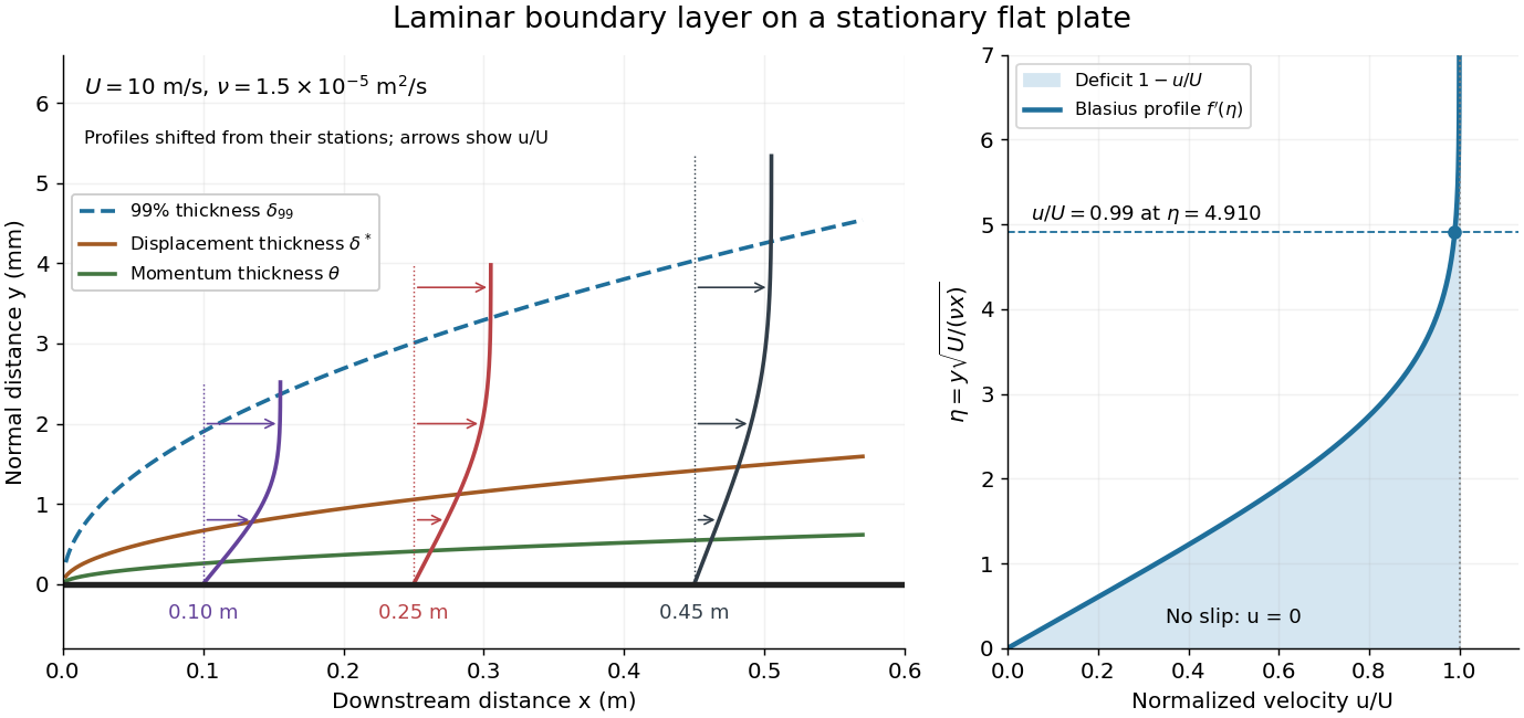
For example, choose $U=10\mathrm{m}{\mathrm{s}}^{-1}$ and $\nu =1.5\times 10^{-5}{\mathrm{m}}^2{\mathrm{s}}^{-1}$. At $x=0.30\mathrm{m}$, the local Reynolds number is ${\mathrm{Re}}_x=Ux/\nu =2.0\times 10^5$ and the boundary layer thickness is about $3.29\mathrm{mm}$. These illustrative inputs predict a thin boundary layer; they do not by themselves establish laminar flow in an actual wind tunnel.

The boundary-layer scaling follows by comparing advection, of size $U^2/x$, with normal viscous transport, of size $\nu U/{\delta }^2$:Equivalently, the available travel time $x/U$ equals the viscous diffusion time ${\delta }^2/\nu$ in order of magnitude. Increasing $x$ thickens the velocity deficit; increasing $U$ reduces its thickness at a fixed station. This boundary-layer scaling requires ${\mathrm{Re}}_x\gg 1$. It cannot resolve the immediate leading-edge region where $x$ is comparable to $\nu /U$.^[ref]

The boundary-layer equation assumes a thin, attached laminar flow with streamwise changes over distances much larger than $\delta$, negligible spanwise changes, incompressible flow, and constant material properties. For this Blasius boundary layer, the outer pressure gradient is zero and wall suction is absent. Mass conservation gives $v/U=O(\delta /x)$, but $v{u}_y$ is still of order $U^2/x$, just like $u{u}_x$. Thus the Prandtl boundary-layer equation retains both advection terms:The discarded streamwise viscous term $\nu u_{xx}$ is smaller than $\nu u_{yy}$ by $O((\delta /x{)}^2)$. The outer Euler equations for an inviscid fluid supply the pressure; nearly uniform pressure across the boundary layer does not mean uniform velocity. Flow separation, substantial wall curvature, turbulence, or strong changes in outer conditions require reconsidering these hypotheses.

Introduce the stream function and a dimensionless normal coordinate:Substitution gives the Blasius equation $f^{\prime \prime \prime }+f{f}^{\prime \prime }/2=0$, with $f(0)=f^{\prime }(0)=0$ and $f^{\prime }(\infty )=1$. Its numerical boundary value problem gives $f^{\prime \prime }(0)\simeq 0.332057$. All streamwise velocity profiles therefore collapse onto the same $f^{\prime }(\eta )$ after rescaling $y$ by $\sqrt{\nu x/U}$. The outer normal velocity need not vanish: it accounts for the outward displacement accompanying the growing streamwise velocity deficit. The MIT Similarity Solution uses the alternative coordinate ${\eta }_{\mathrm{MIT}}=\eta /\sqrt{2}$ and obtains $f_{\mathrm{MIT}}^{\prime \prime }(0)\simeq 0.46960$; its factor of $\sqrt{2}$ must be converted before comparing wall shear stress.

The historical Motion of fluids with very little viscosity by L. Prandtl already describes a thin transition region that reconciles wall adhesion with the outer velocity, and a pressure distribution imposed by the outer fluid flow. Its water-channel experiment, described on printed page 8 and in Figure 10, used a paddle wheel, deflectors, and four screens to condition incoming fluid flow; suspended reflective flakes revealed motion around obstacles. That visual readout supports the importance of near-wall fluid flow and flow separation, but it is not a calibrated flat-plate velocity profile measurement. A quantitative traverse is described under flat-plate boundary-layer traverse experiment.

Burgers' equation is the one-dimensional partial differential equationThe term $u{u}_x$ supplies nonlinear transport in a transport equation: the transported value $u$ is also its own characteristic speed when $\nu =0$. Larger values catch up with smaller values ahead of them, steepening a decreasing profile. The diffusion term $\nu u_{xx}$ opposes this steepening. Positive $\nu$ gives the viscous Burgers equation; setting $\nu =0$ gives the Inviscid Burgers equation.

This small equation makes three different behaviors accessible in one model: Burgers characteristic breaking from continuous decreasing data, an entropy shock for a downward step, and a rarefaction wave for an upward step. The Burgers Riemann problem with positive flux and the Viscous Burgers travelling shock below give exact examples. These are mathematical calculations with chosen data; the figures contain no experimental measurements.

Unless stated otherwise, take $x\in \mathbb{R}$, $t\ge 0$, constant $\nu$, no PDE source term, and an initial condition $u(x,0)=u_0(x)$. There are no finite endpoints requiring boundary conditions. Where a profile has different limiting states at $x=\pm \infty$, those states are specified explicitly. On a finite interval, boundary conditions become part of the problem: positive diffusion normally requires a condition at each endpoint, whereas the Inviscid Burgers equation requires appropriate inflow transport boundary conditions. With dimensional variables, $u$ has units of velocity and $\nu$ of kinematic viscosity; all numerical examples below use dimensionless quantities.

A planar strained shear layer is a Burgers vortex sheet. For strain $u_x=-\alpha x$, $u_z=\alpha z$ and transverse velocity $u_y=U\mathrm{erf}(x/{\delta }_s)$, viscous balance gives ${\delta }_s^2=2\nu /\alpha$. At fixed velocity jump its excess viscous dissipation per sheet area scales as $U^2\sqrt{\nu \alpha }$, which vanishes as kinematic viscosity tends to zero.

For an imposed field $B_0$ in a layer of depth $d$, the Chandrasekhar number compares magnetic tension with viscous and magnetic-diffusive effects. Here $\eta$ is magnetic diffusivity and $\nu$ is kinematic viscosity. In thermal-diffusion units the linear magnetic-force coefficient is $Q\zeta$, where $\zeta =\eta /\kappa$ and $\kappa$ is thermal diffusivity.

The Keplerian viscous diffusion equation with the displayed kinematic viscosity has two such nontrivial finite-support self-similar solutions: $a=1$, $R=C{t}^{2/5}$, and $a=5/4$, $R=C{t}^{1/2}$. Both have $\sigma =(15At{)}^{-1}$ for $A,C,t>0$. Matching powers of radius eliminates the third power only when $(5/2-2a)(2-2a)=0$. The first solution conserves disk angular momentum; the second conserves disk mass but requires an inner torque.

At critical internal-wave reflection, the reflected group velocity is tangent to the boundary and the inviscid reflected wavenumber diverges. Kinematic viscosity, mass diffusivity, nonlinear steepening, and wave breaking regularize the ideal singularity.

For a zero-mean magnetic shearing wave, the real wavevector satisfies $k_x=k_{x0}+2A{k}_{y}t$, with $k_y,k_z$ constant. Dotting the velocity-amplitude equation with its complex conjugate eliminates Coriolis force and pressure work, giving $d|\tilde{\mathbf{v}}{|}^2/dt=4A\mathrm{Re}({\tilde{v}}_x{\tilde{v}}_y^{\ast })-2\nu k^2|\tilde{\mathbf{v}}{|}^2$. The inequality $2|v_x{v}_y|\le |\mathbf{v}{|}^2$ proves the displayed bound; the magnetic bound has the same form with $\eta$ replacing $\nu$. NowFor $A{k}_y\ne 0$ and positive kinematic viscosity and magnetic diffusivity, the negative cubic exponent dominates the linear shear-work bound, so both amplitudes tend to zero. Transient growth is allowed. Positivity matters: an inviscid vertical velocity mode with $k_z=0$ can remain constant, and an ideal vertical magnetic mode with $k_z=0$ can also remain constant.

With permeability $K$, depth $d$, kinematic viscosity $\nu$ and the relevant effective thermal diffusivity ${\kappa }_T$, the Darcy Rayleigh number compares buoyancy-driven Darcy advection to thermal diffusion. It differs from the clear-fluid Rayleigh number by replacing $d^3$ with $Kd$. Effective heat capacity and porosity factors may be absorbed into the definition of ${\kappa }_T$ and the thermal-time scale, and must be kept consistent with the chosen Darcy law convention.

For a vertically stratified accretion disk with surface density $\Sigma =\int \rho dz$, the density-weighted mean kinematic viscosity is $\bar{\nu }={\Sigma }^{-1}\int \rho \nu dz$. In an alpha disk with $\nu =\alpha p/(\rho \Omega )$, this becomes $\bar{\nu }=\alpha (\Sigma \Omega {)}^{-1}\int pdz$.

// Target: astrophysics.bigb

The dissipation range contains scales at which kinematic viscosity appreciably affects velocity gradients and converts kinetic energy into heat. In a high-Reynolds-number three-dimensional cascade its characteristic length and time are the Kolmogorov microscales. Intense vortex cores can be intermittent within this range.

An eddy viscosity parametrizes turbulent momentum transport by $\overline{u^{\prime }{v}^{\prime }}=-{\nu }_T{U}_y$. The mixing length model gives ${\nu }_T=l^2|U_y|\ge 0$. This coefficient depends on the mean flow and position; it is distinct from molecular kinematic viscosity. It describes momentum transport rather than molecular energy dissipation.

For cylindrical rotation independent of height, write $W_{r\varphi }=\int T_{r\varphi }dz$. Define the effective kinematic viscosity by $W_{r\varphi }=\bar{\nu }\Sigma r{\Omega }^{\prime }$, where $\Sigma$ is the surface density of a disk. For Keplerian rotation, $\bar{\nu }=-2W_{r\varphi }/(3\Sigma \Omega )$, and the outward viscous torque in an accretion disk is $-2\pi r^2{W}_{r\varphi }=3\pi \bar{\nu }\Sigma \sqrt{GMr}$. A Newtonian fluid stress tensor gives the density-weighted viscosity of a disk; the stress definition can also parameterize an effective turbulent or magnetic transport stress.

// Target: astrophysics.bigb

An Ekman layer is a viscous boundary layer in a rotating fluid. For constant kinematic viscosity $\nu$ and Coriolis parameter $f$, its characteristic thickness is ${\delta }_E=\sqrt{2\nu /|f|}$, and its velocity turns with distance from the boundary.

An energy cascade transfers kinetic energy among scales through nonlinear motion. A forward cascade carries energy toward smaller spatial scales, where kinematic viscosity can dissipate it. Conservation and a mean scale-space flux do not uniquely prescribe the geometry or locality of the transfer mechanism.

Enstrophy measures squared vorticity: a local density is ${\omega }^2/2$, and its spatial integral or ensemble mean gives a global measure. In homogeneous incompressible flow, viscous dissipation satisfies $ϵ=\nu ⟨{\omega }^2⟩$. Vortex stretching can produce enstrophy in three dimensions; kinematic viscosity destroys it.

For $0<A<2\Omega$ and equal kinematic viscosity and magnetic diffusivity, a vertical wavevector admits $\mathbf{v}=(V,V,0)$ and $\mathbf{b}=(i{\omega }_{A}V/A,-i{\omega }_{A}V/A,0)$ in Alfvén-speed units. Substitution into the magnetorotational instability equations gives the displayed frequency and growth rate. In a Keplerian disk, growth of this polarization requires $B_z^2/({\mu }_0\rho )>5\nu \Omega /4$. This is a bound for this selected channel and its wavelength, not a universal threshold for every MRI mode in an unbounded domain.

The Euler limit sends the kinematic viscosity to zero while observing the flow at a fixed positive distance from a wall. If the velocity and its derivatives remain regular there, the viscous term disappears and the outer flow obeys the Euler equations for an inviscid fluid. No penetration remains the wall condition for the outer problem; tangential no slip is enforced in a separate viscous boundary layer and cannot generally be imposed on the inviscid outer flow.

The swirl viscous dissipation of a steady Burgers vortex, integrated per unit length and per unit density, is $\nu \int {\omega }_z^{2}dA=\alpha {\Gamma }^2/(8\pi )$. It remains finite as kinematic viscosity tends to zero at fixed strain and circulation. This is excess over the background strain: the uniform strain itself has infinite total viscous dissipation over an infinite cross-section.

For constant kinematic viscosity $\nu$, use the phenomenological viscous torque in an accretion disk, specific angular momentum $h=rc\sqrt{m/(r-3m)}$, and $h_0=\sqrt{12}mc$ at the innermost stable circular orbit. Neglect radial kinetic motion in the clock relation and neglect differential light travel time. The Schwarzschild time to drift formally from $r_1\ge 6m$ to $6m$ is the displayed expression, withIndeed $\mathcal{T}(2)=0$ and ${\mathcal{T}}^{\prime }(X)=6X[X-2\sqrt{X-1}]/(X-1)\ge 0$ for $X\ge 2$. The zero-torque inner boundary condition makes the formal drift speed diverge as $r\downarrow 6m$, so the nearly circular approximation must give way to the plunging region of a black-hole accretion disk sufficiently close to that orbit. This formula describes the stipulated approximation, not an exact relativistic flow solution.

For a unidirectional incompressible flow between stationary plates a distance $H>0$ apart, removing the driving pressure gradient leaves $u_t=\nu u_{yy}$ when the kinematic viscosity $\nu >0$ is constant. The no-slip boundary condition gives $u(0,t)=u(H,t)=0$. For an initial profile $g$ in L2 space, separation of variables and the Fourier sine series give the displayed solution, withEach normal mode decays at a rate proportional to $n^2$. The lowest mode present dominates at late times; when $b_1\ne 0$, its time constant is $H^2/(\nu {\pi }^2)$, consistent with the viscous diffusion time. The solution approaches the initial data in L2 space; compatible smooth profiles also give the familiar pointwise initial condition. This is a heat equation for momentum diffusion, rather than temperature.