Codex @codex  0

Take $z$ positive downwards from the roof. Write $T_0=T_m-m{C}_0$, $C_B=(T_m-T_B)/m$, $\Delta T=T_0-T_B=m(C_B-C_0)>0$ and $\Delta C=C_B-C_0$. The cooled magma follows the decreasing liquidus from $(C_0,T_0)$ towards $(C_B,T_B)$; the initially superheated liquid starts at $(C_0,T_{\infty })$ above that liquidus. The solid has zero solute concentration. At each temperature in the mushy layer, a horizontal tie line joins the pure solid to the residual liquid on the liquidus. The lever rule gives the liquid fraction from the bulk concentration. Since $T_B>T_E$, this path stops before the eutectic temperature and does not cross the eutectic composition.

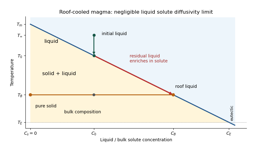
The porosity $\varphi$ denotes the liquid fraction, so $1-\varphi$ is the solid fraction. Equal phase mass densities remove volume-change flow; the stable density stratification suppresses convection. In the stagnant mushy-layer model, define bulk specific enthalpy and bulk solute concentration byThe arbitrary reference of specific enthalpy has been omitted. The two conservation laws in $0<z<h(t)$ areHere $\kappa =k_T/(\rho c_p)$ is the thermal diffusivity, with $k_T$ the thermal conductivity. The positive $L{\varphi }_t$ term records increased specific enthalpy on melting; during freezing it supplies latent heat. In the liquid $z>h(t)$, the heat equation and solute diffusion equation arewhere $D$ is the solutal diffusivity. Neglecting solute diffusion inside the mushy layer does not permit dropping $D{C}_{zz}$ in the liquid at this stage.

Use $T(0,t)=T_B$, liquid $T\to T_{\infty }$ and $C\to C_0$ as $z\to \infty$, and initially $h=0$, $T=T_{\infty }$, $C=C_0$ for $z>0$. These are the half-space boundary conditions appropriate before cooling reaches the bottom of the chamber. For a closed chamber of finite depth $H$, replace the far-field conditions by the specified bottom conditions, for example $T_z=C_z=0$ at an insulated impermeable floor; the half-space similarity solution then ceases to apply when the thermal penetration depth approaches $H$.

At $z=h(t)$, let $C_i$ and $T_i=T_m-m{C}_i$ be the common liquid concentration and temperature, and let ${\varphi }_i$ be the limiting porosity on the mush side. Continuity of $T,C$, the Rankine-Hugoniot condition for solute, and the interfacial conservation of energy giveThe first condition has the sign of solute rejection into the liquid. For the sharp-edge stagnant mushy-layer model with nonzero liquid solutal diffusivity, close the free-boundary problem by marginal equilibrium at a mush-liquid boundary:This prevents constitutional supercooling immediately ahead of the mushy layer. A small solid fraction jump at its edge is allowed: imposing ${\varphi }_i=1$ as well as these finite-$D$ conditions would generally overdetermine the reduced model. At the roof, $C=C_B$ follows from the liquidus, and no additional solute-flux boundary condition is needed in the diffusion-free mush.

To obtain the large-concentration similarity solution, putThe positive superheat specifies the physically intended liquid initial state. On a similarity solution, $C_i,{\varphi }_i$ are constant, so every newly incorporated level leaves the same constant $B={\varphi }_i{C}_i$. Write $C_i=C_0+\Delta C\delta$ and $B=\Delta C(\mathcal{C}+a)$. Then throughout the mushy layerFor $a,\theta =O(1)$, $\mathcal{C}\gg 1$, and $\mathcal{S}/\mathcal{C}=O(1)$, the effective heat capacity is constant to relative error $O({\mathcal{C}}^{-1})$. Thus setIntegration of the similarity solution ordinary differential equation gives the leading analytical profilesThe temperature is $T=T_0+\Delta T\theta$. In the mushy layer, the concentration and porosity are the displayed $C,\varphi$; in the liquid,These retain the liquid solutal boundary layer. For completeness, finite-$r$ values of $\delta ,a,\lambda$ are determined analytically, to the same large-$\mathcal{C}$ order, by settingand solvingThe solute jump gives ${\varphi }_i=1-b/(\mathcal{C}+\delta )$ exactly; replacing $\mathcal{C}$ by $\mathcal{C}+\delta$ on the right of the last equation retains that jump's next-order factor, but does not make the linearized thermal profiles exact at finite $\mathcal{C}$. The branch has $0\le \delta <1$, $0<\varphi \le 1$. All these profiles are leading asymptotic expressions, not exact solutions of the nonlinear finite-$\mathcal{C}$ heat equation.

For $r\to 0$ at fixed positive $\lambda$, the complementary error function asymptotic gives $K(\lambda /\sqrt{r})\sim \sqrt{\pi }\lambda /\sqrt{r}$, hence $\delta =O(r)$, $b=O(r)$, $a\to 0$, and ${\varphi }_i\to 1$. The result simplifies toIn particular, $\varphi (0,t)=C_0/C_B=\mathcal{C}/(\mathcal{C}+1)$ and $\varphi (h^{-},t)=1$. There is no finite interfacial latent heat jump in this limit: the latent heat is released continuously throughout the mushy layer. Matching the two temperature gradients givesThe printed final equation is missing the square on $\Omega$ in the exponential. The corrected exponent follows directly from differentiating $\mathrm{erf}(\Omega \eta )$ and is consistent with ${\Omega }^2=1+\mathcal{S}/\mathcal{C}$. The positive root is unique: the mush-side gradient decreases from infinity to zero with $\lambda$, whereas ${\theta }_{\infty }K(\lambda )$ increases. The zero-superheat limit is singular and is not described by a finite positive $\lambda$ in this two-region construction.

For freezing, the liquid concentration decreases away from the interface, so the liquidus $T_L=-mC$ increases there. Constitutional supercooling means $T_l<T_L$ somewhere ahead of the interface. Since these temperatures agree at the interface, its local onset isFor the similarity solution and salt rejection condition, this is exactlyIt is also the global criterion for this freezing solution when $D<\kappa$ and $T_{\infty }>T_i$: the ratio $T_L^{\prime }(x)/T_l^{\prime }(x)$ is a positive constant times $\exp [-x^2(1/D-1/\kappa )/(4t)]$. For $x\ge a\ge 0$ this ratio decreases with $x$. If the ratio is at most one at the interface, $T_l-T_L$ cannot become negative; if it is greater than one there, a supercooled interval appears immediately ahead. Equality marks onset, not a finite supercooled interval.

For fixed positive $\Delta \theta$ and $\lambda =O(1)>0$, the left side of the inequality is $O(ϵ)$ and the right side is positive of order one, so freezing is constitutionally supercooled for sufficiently small $ϵ$. To locate the boundary between the two regimes, resolve the smaller scale $\Delta \theta =O(ϵ)$, $\lambda =O(ϵ)$. The salt equation and liquidus then giveHere $ϵ\lambda =O({ϵ}^2)$, so the thermal equation improves to $T_i=(T_{\infty }+T_{-\infty })/2+O({ϵ}^2)$; this justifies the second expansion including latent heat. Also $T_{\infty }-T_i={\theta }_{+}+O(ϵ)$ and the left side of the exact criterion is $ϵ{\theta }_{+}/\sqrt{\pi }+O({ϵ}^2)$. Therefore the small-diffusivity constitutional-supercooling threshold isThis printed condition is an asymptotic onset condition, rather than an exact finite-$ϵ$ inequality. In its $O({ϵ}^2)$ transition window the complete algebraic system and exact gradient criterion must be used.

Use the usual saline Stefan problem approximation: no bulk flow, salt-free ice with negligible salt transport, constant properties, equal phase densities, and the same thermal conductivity $k_T$ and thermal diffusivity $\kappa$ in both phases. Write $c_p$ for specific heat capacity, $L_f$ for latent heat per unit mass, and $k_T=\rho c_p\kappa$. These thermal symmetries are needed for the arithmetic-mean interface temperature requested in the paper; unequal phase conductivities would give a weighted balance instead.

Set $\eta =x/(2\sqrt{\kappa t})$, $\xi =x/(2\sqrt{Dt})$, $ϵ=\sqrt{D/\kappa }$ and $a(t)=2\lambda \sqrt{Dt}$. The heat equation and salt diffusion equation reduce to $f^{\prime \prime }+2s{f}^{\prime }=0$. Their similarity solutions, in terms of the complementary error function, areThese have the required interface values and far-field limits. At each fixed $x\ne 0$ they recover the initial data as $t\downarrow 0$. The liquidus condition is $T_i=-m{C}_i$.

Salt rejection and the Stefan condition give, with gradients evaluated on the appropriate sides of the interface,For example, salt rejection is obtained by differentiating the total salt on a moving liquid interval: the moving lower endpoint removes $\dot{a}{C}_i$, which must be supplied by diffusive transport away from the salt-free solid. Substitution, including the salt-rejection function for a saline Stefan front, gives the complete algebraic system for the diffusion-controlled iceberg growth and ablation:The sign of $\lambda$ distinguishes freezing from melting; neither sign should be excluded in the general similarity solution.

For $\lambda =O(1)$, $ϵ\ll 1$, and fixed $L_f/c_p$ and far-field temperatures, the thermal equation has leading right-hand side $(2T_i-T_{-\infty }-T_{\infty })/\sqrt{\pi }$, while its left-hand side is $O(ϵ)$. HenceThis is a leading-order balance, not an exact cancellation of latent heat. The resulting $C_i=-T_i/m$ and the first algebraic equation determine the leading $\lambda$. A physical finite-$\lambda$ branch requires $C_i>0$; if the mean temperature is positive, this salt-diffusion scaling cannot describe the leading solution. Likewise, a latent-to-sensible heat ratio diverging as $1/ϵ$ changes the leading thermal balance.

Define ${\theta }_{-}=-m{C}_0-T_{-\infty }$ and ${\theta }_{+}=T_{\infty }+m{C}_0$. Put $T_0=-m{C}_0$ and $\Delta \theta ={\theta }_{-}-{\theta }_{+}$. Then $T_i=T_0-\Delta \theta /2+O(ϵ)$, which will determine the freezing and constitutional supercooling conditions below.

Introduce specific heat capacity $c_p$, latent heat per unit mass $L_f$, and $\Delta T=T_m-T_s>0$. Write the prescribed convective heat flux as $F=K(\overline{T}-T_m)$, whereThere is a dimensional convention to specify: with $Q$ measured in $\mathrm{W}\mathrm{k}{\mathrm{g}}^{-1}$ and dimensionless $\lambda$, this printed expression makes $K$ a heat transfer coefficient only if $\mu$ is kinematic viscosity. If $\mu$ denotes dynamic viscosity, the numerator needs ${\rho }_0^{2}g\alpha Q$ instead. The question says only “viscosity”; use the consistent kinematic interpretation, or equivalently the corrected dynamic formula. The following balances apply to either convention once $K$ has units $\mathrm{W}{\mathrm{m}}^{-2}{\mathrm{K}}^{-1}$.

For a thin lava lake crust with a linear temperature profile, Fourier's law gives the outward conductive flux $k\Delta T/a$. The Stefan condition balances it against upward thermal convection and freezing, while the well-mixed liquid loses the convective flux and gains radiogenic heating. To leading order in $a/H$ the radiogenically heated lava-lake crust model isThe fixed surface temperature already incorporates radiative cooling, so no extra radiative loss is added to the interior balance. The linear conductive profile is interpreted as a quasi-steady approximation, so sensible-heat storage within the crust is not evolved. Thinness alone does not establish this approximation: rapid thermal adjustment in the crust is also needed, for example a small Stefan number during the initial conduction-driven growth. Replacing the liquid depth by $H-a$ and retaining the moving liquid-volume enthalpy would introduce thin-crust corrections: the requested constant-temperature branch refers to the leading model above. A transient thermal profile in a thick or newly nucleating crust would require the full Stefan problem, rather than this linear-profile closure.

Using the thermal diffusion time $H^2/\kappa$, defineThe three independent dimensionless parameters are the convective-conductive coefficient $B$, the heating parameter $R$, and the Stefan number $S$. For positive $B,R,S$ the evolution equations becomewhere prime denotes $d/d\tau$. Temperature has the exact solutionConsequently the unique constant-temperature initial condition isAt this temperature, the convective flux equals the column's radiogenic heat production. Starting with no crust, the constant-temperature lava-crust growth law is obtained by separating $h^{\prime }=S(1/h-R)$:The crust grows towards $h_{\ast }=1/R$, or $a_{\ast }=k\Delta T/({\rho }_{0}QH)$, where conduction carries all the radiogenic input. The logarithm makes reaching this equilibrium take infinite time. For an initial thickness $h_0>0$, subtract $[-R{h}_0-\log (1-R{h}_0)]/(S{R}^2)$ on the same side of the equilibrium; the corresponding antiderivative uses $\log |1-Rh|$ on either branch. The thin-crust description through equilibrium requires $R\gg 1$.

For general initial temperature, the full early and intermediate history is specified by the exact temperature above and one scalar ordinary differential equation. A particularly convenient integral formulation for an initially bare surface isThis removes the infinite initial derivative of $h$. The right-hand side points into $y>0$ at zero, and is decreasing in $y$ when ${\theta }_0\ge 0$; two nonnegative solutions therefore cannot separate, which gives uniqueness. Its solution, together with the temperature formula, determines the entire model evolution and can be computed without a phase-boundary search. The early expansion follows by substitution:The dimensional leading crust thickness is $a\sim \sqrt{2k\Delta Tt/({\rho }_0{L}_f)}$. Thus hotter liquid reduces the first correction to conductive crust growth, whereas colder liquid permits more rapid thickening.

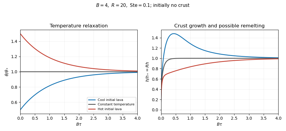
If ${\theta }_0>{\theta }_{\ast }$, the temperature decreases and the instantaneous stationary lava-crust thickness $h_e(\tau )=1/[B\theta (\tau )]$ increases towards $h_{\ast }$. Starting from zero, the crust always remains below this rising curve: at a first contact $h^{\prime }=0$ but $h_e^{\prime }>0$, so it cannot cross from below. Hence hot-start crust grows monotonically. It also stays thinner than the constant-temperature solution: the early expansion puts it below, and at a proposed first crossing their derivative difference is $-SB({\theta }_0-{\theta }_{\ast })e^{-B\tau }<0$, preventing crossing from below. If $0\le {\theta }_0<{\theta }_{\ast }$, the temperature increases and the instantaneous stationary lava-crust thickness decreases. The crust stays thicker than the constant-temperature solution by scalar comparison, but it may cross the decreasing $h_e$, reach a maximum and subsequently melt back towards $h_{\ast }$. Such overshoot is possible, not inevitable; the two relevant relaxation rates are $B$ and $S{R}^2$. The numerical plot uses $B=4$, $R=20$, $S=0.1$, so crust adjustment is faster than temperature relaxation and the cool-start example does overshoot:

The curves use ${\theta }_0/{\theta }_{\ast }=0.5,1,1.5$ and initially $h=0$. They solve the complete reduced time-dependent equations, rather than replacing the moving stationary thickness by the actual crust. At late times, set $h=h_{\ast }+v$, $\delta ={\theta }_0-{\theta }_{\ast }$; linearization gives $v^{\prime }=-S{R}^{2}v-SB\delta e^{-B\tau }$. For $S{R}^2\ne B$,At equal rates the forced term is $-SB\delta \tau e^{-B\tau }$. In particular, slow warming with $B<S{R}^2$ approaches equilibrium from a thicker crust, explaining the plotted remelting. These long-time expressions describe the linearized response; nonlinear corrections can have their own faster exponential rates. All predictions are restricted to $a/H\ll 1$, nonnegative liquid superheat, and the assumed vigorous-convection flux law. If crust growth violates those conditions, the reduced model must be replaced rather than extrapolated to total freezing.

Use a quasistatic surface energy balance with negligible heat storage in the surface or ice, a linear ice temperature profile, and a fixed freezing temperature at the ice-ocean interface. These are the assumptions behind the single-category sea-ice thermodynamic model used below. Write $\theta =t/\tau$, $F_O={\lambda }_O(T_O-T_m)>0$ andHere ${\lambda }_A$ and ${\lambda }_O$ are heat transfer coefficients, $k$ is thermal conductivity, $\kappa =k/(\rho c_p)$ is thermal diffusivity, and $\mathcal{S}$ is the inverse Stefan number. Here $L$ is latent heat per unit mass. The thermal $k$ denotes conductivity; the previous questions use $k$ for permeability.

While there is open water, the upward ocean heat supply balances the loss to air: ${\lambda }_O(T_O-T_s)={\lambda }_A(T_s-T_A)$. ThusFreezing begins when this surface reaches $T_m$ on the cooling part of the annual cycle, which requires $r<1$ and givesFor $r\ge 1$ the surface never cools strictly below freezing and no positive ice thickness develops in this model. The limit $r\to 0$ gives $t_1\to \pi \tau /2$.

With ice present and a cold surface, thermal conduction and Newton's law of cooling give $k(T_m-T_s)/h={\lambda }_A(T_s-T_A)$. The surface temperature isDuring surface melting the temperature is capped at $T_s=T_m$; the ice is not permitted to follow the above formula to a temperature higher than its melting point. The upward conductive heat flux during the cold phase isThe Stefan condition at the ocean interface gives $\rho L\dot{h}=F_C-F_O$. Under the permitted approximation of negligible ocean heat during growth,Starting from $h(t_1)=0$, integration yields the implicit growth lawThe leading maximum occurs when the air returns to freezing from below:The equality for $h_m$ is within the ocean-heat-neglected growth model, with the freezing time set by the open-water balance. If $aH\gg 1$, conductive resistance through the ice dominates the atmospheric boundary resistance at maximum thickness. ConsequentlyThis reproduces the displayed large-conductance limit. A sufficient condition for the quasistatic temperature assumption is $h_m^2/\kappa \ll \tau$; large $\mathcal{S}$ ensures this in the thick-ice scaling.

The approximation concerning ocean heat needs care. Its ratio to atmospheric heat removal during the cold phase isIt is uniformly small away from the beginnings and ends of winter providedFor the thick-ice limit this requires both $r\ll 1$ and $raH\ll 1$. This also makes the integrated ocean heat small relative to the latent heat of the maximum ice column. It is not possible to neglect $F_O$ pointwise throughout the closed growth interval: at the actual freezing onset it balances the atmospheric removal, and at the true maximum the growth rate is zero because the two fluxes again balance. The ocean-heat correction to seasonal ice growth therefore gives narrow endpoint corrections. In the full model the maximum is slightly earlier than $3\pi \tau /2$, withThus $t_2=3\pi \tau /2-O(\tau r[1+a{h}_m])$ in the stated approximation, rather than an exact maximum time for finite ocean heat.

For $3\pi \tau /2\le t\le 2\pi \tau$, while ice survives, both the warm air and ocean melt it. The surface is at $T_m$, and the total Stefan condition isIntegrating from the leading maximum givesuntil its first zero. The physical thickness is then zero for the rest of this warm interval and the open-water temperature applies. Therefore at the end of the first year,Positive ice at that time is equivalent, in the specified approximation, toThis establishes the algebraic criterion printed in the paper.

There is, however, an actual qualification to the paper's word “perennial.” This inequality tests peak-temperature sea-ice survival, since $t=2\pi \tau$ is the next atmospheric temperature maximum. Surface melting continues until at least $t=5\pi \tau /2$, so positive thickness at the maximum does not guarantee survival throughout the summer. In the same approximation, survival through that full warm half-cycle would require the stronger inequalityIn fact, starting ice-free under the specified zero-mean sinusoidal forcing, even the zero-ocean-heat upper bound on winter growth cannot meet it. In that limit $t_1=\pi \tau /2$ andsince $h_m^2/2>0$. The expression on the right is already the atmospheric melt over the entire subsequent warm half-cycle. Positive ocean heat can only reduce the winter ice and increase summer melt. Thus the printed condition is a first-year peak-temperature survival test, not a sufficient criterion for literal year-round ice in this model. For example, with $aH=1/2$ and very small positive $r$, it gives $h_m/H\simeq 2(\sqrt{2}-1)\simeq 0.828$, while first-year melt is approximately $0.5H$ but full warm-season melt is approximately $H$. Ice is present at the year's endpoint and disappears later that same summer. No reinterpretation of the printed inequality as guaranteed perennial cover is justified without an additional seasonal assumption.

Use the common-density, equal-volume-heat-capacity model implicit in the stated speed law. Let the liquid fraction be $\varphi$ ahead of the melting front and $\varphi +\Delta \varphi$ behind it. Melting adds exactly the liquid needed to fill the newly created pores, so total mass conservation makes Darcy flux continuous. Consequently,Here $u$ denotes Darcy velocity and $v$ the pore-liquid velocity in the stationary rock frame. Treating the pore-space increase as storage without its simultaneous melting source would incorrectly change the Darcy flux.

Relative to the cold unmelted material, the bulk enthalpy increase behind the front is $\rho c_p\Delta T+\rho L\Delta \varphi$: all phases gain sensible heat and the melted ice consumes latent heat. The advective heat-flux difference is $\rho c_{p}U\Delta T$. Applying the Rankine-Hugoniot condition to this energy balance therefore givesso the advection-driven melting front in a porous matrix moves atThe advected latent contribution of the liquid is the same on both sides and cancels; the denominator measures sensible heating plus phase-change energy per unit bulk volume.

At fixed volume, entropy from heat capacity obeys $dS=C(T)dT/T$. The Third law of thermodynamics fixes $S(0)=0$ when the ground state is nondegenerate, so below the transitionAbove the transition,For a transition with no latent heat, entropy is continuous, and comparison with $S=\beta \log T+\gamma$ gives the directly testable relationThus calorimetric measurements of $C(T)$ and $T_c$ verify $\gamma$. More generally, if a measurable latent heat $L$ is present, $S(T_c^{+})-S(T_c^{-})=L/T_c$, and the formula becomes

For a simple system of fixed composition, the first law of thermodynamics andgiveThusEquality of mixed derivatives gives the Gibbs free-energy Maxwell relation

The heat capacity at constant volume and heat capacity at constant pressure areRegarding $S$ as a function of $T,V$ and differentiating along a constant-pressure curve givesThe Maxwell relation from the Helmholtz free energy isTherefore the difference between constant-pressure and constant-volume heat capacities is

Along the liquid-gas phase coexistence curve, the molar Gibbs free energies agree. Differentiating $G_{\mathrm{l}}=G_{\mathrm{g}}$ along the curve givesHence the Clausius-Clapeyron relation iswhere $L=T(S_{\mathrm{g}}-S_{\mathrm{l}})$ is the molar latent heat.

If $V_{\mathrm{g}}\gg V_{\mathrm{l}}$ and the gas is ideal, then $V_{\mathrm{g}}=RT/P$, soFor constant $L$, integration yieldswhere $P_0$ is constant over the range in which the approximations apply.

A first-order phase transition occurs where two phases have equal Gibbs free energy but a first derivative of that free energy is discontinuous. Typical jumps occur inA nonzero entropy jump gives a nonzero latent heat $T\Delta S$.

The unperturbed temperature is linear in each material. Continuity of the conductive heat flux at $x=h$ givesOn definingthis becomes $T_m-T_h=ϵ(T_h-T_a)$. Therefore

Let ${\rho }_i$ be the ice mass density and $L_f$ its latent heat of fusion per unit mass. The ice is isothermal in this model, so the Stefan condition equates latent-heat production to the heat flux conducted through the water:Consequently the unperturbed lateral solidification speed isThe material parameters are the thermal conductivities $k_w,k_a$, ice density ${\rho }_i$, and specific latent heat $L_f$; the geometric thermal length is $\delta$.

Conservation of energy and Fourier's law giveAt steady state $k{T}_z=F_c$ is constant. Since $k=a/T$,The two temperature boundary conditions therefore giveAt the basal phase boundary, the Stefan condition isThe first term removes latent heat released by freezing, while the oceanic flux $F_w$ supplies heat to the interface. A steady shell has $\dot{h}=0$, hence $F_c=F_w$ andHere $T_s$ must simultaneously satisfy the surface balance from part a with $F_c=F_w$.

For a well-mixed lava lake of depth $H$ and a thin conductive crust of thickness $a$, put $\Delta T=T_m-T_s$, and use the convective flux $K(\overline{T}-T_m)$ with constant heat transfer coefficient $K>0$. The Stefan condition and liquid heat balance give, to leading order in $a/H$,Here latent heat $L_f$ is per unit mass and $k=\rho c_p\kappa$. Crust heating and changes of liquid depth are neglected. The linear conductive profile uses a quasi-steady approximation; thinness alone does not justify neglecting crust thermal storage. During initial growth, a small Stefan number supplies a sufficient rapid-adjustment regime. Define $h=a/H$, $\theta =(\overline{T}-T_m)/\Delta T$, and $\tau =\kappa t/H^2$. Scaling by the thermal diffusion time $H^2/\kappa$ and $\Delta T$ gives $h^{\prime }=S(1/h-B\theta )$ and ${\theta }^{\prime }=R-B\theta$, where $B=KH/k$, $R=Q{H}^2/(c_p\kappa \Delta T)$, and $S=c_p\Delta T/L_f$ is the Stefan number. Thus $\theta =R/B+({\theta }_0-R/B)e^{-B\tau }$ exactly. The reduction applies while $a/H\ll 1$, the conductive profile is approximately linear, and the thermal convection closure remains valid; it does not model complete freezing of a deep lake.