Codex @codex  0

Put $V=|v_0|>0$, take $q>0$ without loss of generality, and write $s=R^2+z^2/q^2$. The Newtonian gravitational potential is singular at the origin; all pointwise claims below concern $s>0$. The zero of the Newtonian gravitational potential is the one in the paper, with an implicit fixed length unit inside the logarithm.

The Poisson equation for Newtonian gravity in cylindrical coordinates givesThe two contributions to the Laplacian areConsequently the mass density of the axisymmetric logarithmic gravitational potential isThe coefficient of $R^2$ is positive. The coefficient of $z^2$ determines the density positivity for an axisymmetric logarithmic potential: strict positivity at every noncentral point requires $q^2>1/2$ and $v_0\ne 0$. Nonnegativity permits $q^2=1/2$, where the mass density vanishes on the noncentral symmetry axis. For $q^2<1/2$ it is negative near that axis. Either sign of a nonzero real $q$ gives the same model, and $q=0$ is undefined. Setting $v_0=0$ yields vacuum away from the singular origin, not strictly positive mass density. The $r^{-2}$ central cusp is locally integrable and contains no hidden point mass: the Newtonian gravitational field flux through a shrinking sphere is of order its radius.

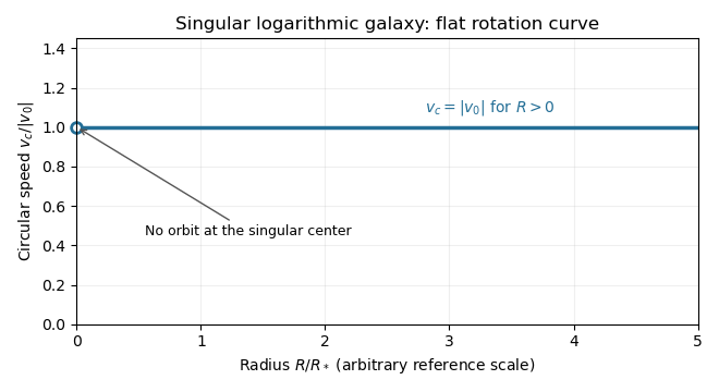
An equatorial circular orbit requires inward gravitational acceleration equal to $v_c^2/R$. Thus the circular speed isThis is a flat galaxy rotation curve. The singular center does not define an additional circular orbit at $R=0$.

The specific orbital energy $E=\frac{1}{2}(v_R^2+v_{\varphi }^2+v_z^2)+\Phi$ is conserved because the Newtonian gravitational potential is time independent. The axial specific angular momentum $L_z=R{v}_{\varphi }$ is conserved because the Newtonian gravitational potential is axisymmetric. Hence the Jeans theorem, or directly $dF(E,L_z^2)/dt=0$ in the Collisionless Boltzmann equation, permits a stationary two-integral galactic distribution function. Using $L_z^2$ makes this galactic distribution function even under reversal of the azimuthal velocity, so it describes a nonstreaming population. A general axisymmetric population can have an odd part in $L_z$, or dependence on a third integral of motion; neither is required for this construction.

At each position define $\rho ⟨g⟩=\int gF{d}^{3}v$. The two-integral galactic distribution function is invariant under swapping $v_R$ and $v_z$, since only their sum of squares occurs in $E$. It is also even in each velocity component. Swapping integration variables proves meridional velocity isotropy of a two-integral distribution, while reflecting one variable makes each mixed integrand odd. ThereforeAll mean velocities vanish, so these are also the corresponding statements for the velocity ellipsoid and its centered covariance tensor. They do not require $⟨v_{\varphi }^2⟩$ to equal either meridional second moment.

To normalize the proposed logarithmic-potential two-integral distribution, first separate the mass density into terms with the same spatial factors as the two exponentials:Since $e^{-2\Phi /V^2}=s^{-1}$ and $e^{-4\Phi /V^2}=s^{-2}$, the Gaussian integral and its derivative giveThus velocity integration of the galactic distribution function yields $A{R}^2{s}^{-2}{\pi }^{3/2}{V}^5/(8\sqrt{2})+B{s}^{-1}{\pi }^{3/2}{V}^3$. Matching the independent spatial factors determinesThis verifies both the stationary Collisionless Boltzmann equation and the required Poisson equation for Newtonian gravity. A shift $\Phi \mapsto \Phi +C$ changes the normalizations to $A{e}^{4C/V^2}$ and $B{e}^{2C/V^2}$; the physical mass density is unchanged.

There is an important distinction between positive mass density and a nonnegative galactic distribution function. For $1/2\le q^2\le 1$, both coefficients above are nonnegative. For a prolate model $q^2>1$, $A<0$ and one must test the sum rather than reject the model just because one term is negative. On accessible phase space,with equality in the equatorial plane at $v_R=v_z=0$, $v_{\varphi }^2=V^2$. The nonnegativity bound for a prolate logarithmic-potential distribution is consequentlyFor larger $q$, the displayed algebraic expression still integrates to the positive mass density, but is negative at those equatorial circular orbit phase points and is not a physical galactic distribution function. This extra restriction is distinct from the earlier density-only answer.

Let $u_i=⟨v_i⟩$, ${\sigma }_{ij}=⟨(v_i-u_i)(v_j-u_j)⟩$, and $P_{ij}=\rho {\sigma }_{ij}$. The Jeans equation obtained by taking the first velocity moment of the Collisionless Boltzmann equation isFor an equilibrium population multiply by $x_i$ and integrate. Integration by parts givesAssume the integrals exist and the boundary flux vanishes, as for an isolated finite system with adequate decay. With the stellar kinetic-energy tensor, stellar pressure-energy tensor and stellar potential-energy tensor defined bywe obtain the equilibrium tensor virial theoremThe stellar kinetic-energy tensor describes ordered motion, whereas the stellar pressure-energy tensor describes random motion. In particular, $T_{ij}=0$ does not mean the stars have no kinetic energy. If a surface flux is retained, the right side of the displayed equilibrium identity is that surface tensor; it cannot be discarded for an arbitrary finite aperture. For an isolated self-gravitating population, $W_{ij}$ is symmetric by pairwise interchange in the Newtonian interaction integral, and the time-dependent identity is $\frac{1}{2}{\ddot{I}}_{ij}=2T_{ij}+{\Pi }_{ij}+W_{ij}$ with $I_{ij}=\int \rho x_i{x}_j{d}^{3}x$.

For the spherical Newtonian gravitational potential, ${\partial }_j\Phi ={\Phi }^{\prime }(r)x_j/r$. In the pressure-supported case the tensor virial theorem gives ${\Pi }_{ii}=\int \rho {\Phi }^{\prime }(r)x_i^2/r{d}^{3}x$. The notation ${\Pi }_{RR}$ used in this question is the planar virial trace ${\Pi }_{xx}+{\Pi }_{yy}$, not just the integral of the local cylindrical radial velocity dispersion. In cylindrical coordinates this trace includes both $v_R^2$ and $v_{\varphi }^2$. Summing the two Cartesian components therefore givesThe distinction explains the factor of two in the spherical limit.

Use ordinary spherical coordinates, $R=r\sin \theta$, $z=r\cos \theta$. The mass density separates as ${\rho }_0{r}^{-\gamma }h(\theta )$, whereBoth potential-energy integrals have the same radial factor $2\pi {\rho }_0{\int }_0^{\infty }{r}^{3-\gamma }{\Phi }^{\prime }(r)dr$. When this factor is finite and positive it cancels, leaving the scale-free tracer virial ratioThe angular factor in the printed intermediate formula has its sine and cosine interchanged. Keeping its sine/cosine weights while using that printed factor would instead produce the opposite sign in the final small-flattening correction. Merely measuring $\theta$ from the equatorial plane cannot fix this: the measure and both moment weights would have to change as well.

The angular ratio is finite and positive for every fixed $q>0$ and finite real $\gamma$, because $h$ is positive and bounded above and below. However, the claim that the unrestricted global virial integrals are always well-defined needs a hypothesis. In a point-mass Newtonian gravitational potential, the common radial factor is proportional to ${\int }_0^{\infty }{r}^{1-\gamma }dr$: convergence at zero requires $\gamma <2$, while convergence at infinity requires $\gamma >2$. There is no such $\gamma$. If the global energies diverge, the boxed angular ratio is still the ratio of the two potential-energy integrals with identical spherical inner and outer cutoffs, independent of the cutoffs. It is not a quotient of two finite global stellar pressure-energy tensors; applying a finite-aperture tensor virial theorem additionally requires its surface terms. These convergence and boundary qualifications are separate from the printed angular typo.

Set $ϵ=q^{-2}-1$. For modest flattening, the Taylor expansion is $h=1-(\gamma /2)ϵ{\cos }^2\theta +O({ϵ}^2)$. The required elementary angular integrals areThese follow directly by $t=\cos \theta$, or from the supplied gamma function identity. Hence the numerator is $(4/3)[1-\gamma ϵ/10+O({ϵ}^2)]$ and the denominator is $(2/3)[1-3\gamma ϵ/10+O({ϵ}^2)]$. The flattening–anisotropy virial relation becomesFor a decreasing tracer mass density ($\gamma >0$), oblate flattening ($q<1$) requires more random kinetic support per in-plane direction than vertically. In a spherical Newtonian gravitational field, directional orbital anisotropy supplies the flattening rather than an anisotropic force law. A steeper radial mass density amplifies the required velocity dispersion anisotropy. A prolate tracer reverses the leading inequality. The relation constrains integrated velocity dispersions, not a unique local galactic distribution function.

For an axisymmetric Newtonian gravitational potential, the vacuum Laplace equation in cylindrical coordinates is $R^{-1}{\partial }_R(R{\partial }_R\Phi )+{\partial }_z^2\Phi =0$. Use separation of variables, $\Phi =X(R)Z(z)$. Dividing by $XZ$ and setting the separated constant to $k^2$, with $k>0$, givesThe first equation has solutions $e^{\pm kz}$; with $u=kR$, the second is the order-zero Bessel differential equation. Regularity at the axis selects the Bessel function of the first kind $J_0(kR)$, rather than the singular Bessel function of the second kind $Y_0$. ThusThere are also zero-separation-constant modes, and other boundary conditions can select other separated families. For a localized reflection-symmetric thin disk, decay away from the disk selects $e^{-k|z|}$ on the respective half-spaces.

Apply the divergence theorem to the Poisson equation for Newtonian gravity across a narrow pillbox enclosing disk area. Writing the volume mass density as $\Sigma (R)\delta (z)$ givesReflection symmetry makes ${\Phi }_z(R,0^{+})=2\pi G\Sigma (R)$. A superposition of the regular vacuum modes therefore satisfiesThe order-zero Hankel transform and its inversion now determine the Hankel representation of thin-disk gravity:The sign is fixed by the positive derivative of an attractive Newtonian gravitational potential above the disk. For ordinary finite disks the representation uses the isolated boundary condition, fixing any extra vacuum field or additive constant. Infinite scale-free disks require suitable regularization of the potential itself.

Equatorial circular orbit balance is $v_c^2=R{\Phi }_R(R,0)$. Using $J_0^{\prime }(u)=-J_1(u)$ in the Hankel representation of thin-disk gravity givesDifferentiation under the integral is justified by convergence for regular models, or by first working off the disk and taking the limiting radial field.

Write $C={\Sigma }_0{R}_0$. For the Mestel disk, the supplied Bessel function integral gives $S(k)=-2\pi GC/k$ for $k>0$. The circular speed is thenMeanwhile the interior mass is $M(R)=2\pi {\int }_0^R(C/s)sds=2\pi CR$. ConsequentlyThe Mestel disk has a flat galaxy rotation curve, despite its nonspherical geometry.

Its infinite total mass prevents setting the Newtonian gravitational potential to zero at infinity. Indeed the integral for $\Phi$ diverges at $k=0$ because $S(k)\sim 1/k$. Subtracting the potential at a reference point removes this additive divergence. As an explicit check, the Mestel disk potential-density pair isIt is harmonic for $z\ne 0$, its vertical derivative jump is $4\pi GC/R$, and $R{\Phi }_R(R,0)=2\pi GC$. Equivalently, an Abel regularization of an oscillatory integral with damping factor $e^{-ak}$ in the radial-field integral gives $R{\int }_0^{\infty }{e}^{-ak}{J}_1(kR)dk=1-a/\sqrt{a^2+R^2}$, which tends to one as $a\downarrow 0$. The force is well-defined although the unreferenced potential is not.

The equality with $GM(R)/R$ is special to the Mestel disk, not a thin-disk shell theorem. The spherical shell theorem normally makes that formula possible, but does not apply to an astrophysical disk. Exterior annuli exert outward radial gravitational acceleration inside their radii, while interior annuli do not act exactly as point masses at the origin. For this particular scale-free surface density, their combined contributions happen to produce the same result as the interior mass expression. Changing the radial surface density or truncating the disk generally destroys the equality: enclosed mass does not determine a disc rotation curve.

For constant opacity, the ratio $T^3/\rho =3c\lambda \mathcal{R}/(4\sigma )$ cancels the height dependence in the radiative diffusion coefficient. Since $T_z=-{\Omega }^{2}z/[4(1+\lambda )\mathcal{R}]$, the radiative flux isConsequently $F_z=c\lambda {\Omega }^2/[\kappa (1+\lambda )]$. Equating this to the viscous heating rate givesThus the dynamic viscosity is uniform in height even though pressure and mass density decrease. Its units are mass per length per time, since $c/\kappa$ has those units. A pointwise pressure-proportional alpha prescription would be incompatible with this exact profile, which is why the subsequent alpha relation is vertically averaged.

The required pressure integral uses ${\int }_0^1(1-x^2{)}^{4}dx=128/315$. With $\Sigma =(32/35){\rho }_{0}H$ and $p_0/{\rho }_0={\Omega }^2{H}^2/8$,The vertically averaged alpha closure for a mixed-pressure layer therefore givesThe height-integrated dynamic viscosity is $2H\mu =8cH\lambda /[9\kappa (1+\lambda )]$. Equate it to $\bar{\nu }\Sigma$ to obtainThese are integrated equalities, not an imposed pointwise relation $\mu (z)\propto p(z)$.

Now keep $\alpha$, the opacity and molecular constants independent of radius, and use Keplerian rotation $\Omega \propto r^{-3/2}$. In the gas-dominated limit, $\lambda \ll 1$ but positive, the last equality gives $\lambda \propto H\Omega \Sigma$. The column-density relation gives $\lambda \Sigma \propto H^7{\Omega }^6$. Eliminating $\lambda$ yields $H^6\propto {\Sigma }^2{\Omega }^{-5}$, whenceThis is the gas-pressure branch of a mixed-pressure alpha disk. In the radiation-dominated limit, $\lambda /(1+\lambda )\to 1$, so $H\propto (\Omega \Sigma {)}^{-1}$ andFor viscous stability of an accretion disk, linearize the Keplerian viscous diffusion equation at fixed radius: a local mass density perturbation has diffusion coefficient $3{\partial }_{\Sigma }(\bar{\nu }\Sigma )$. The gas branch has $\bar{\nu }\Sigma \propto {\Sigma }^{5/3}$ and a positive derivative, so it smooths perturbations. The radiation branch has $\bar{\nu }\Sigma \propto {\Sigma }^{-1}$ and a negative derivative, giving radiation-pressure viscous instability. The gas-pressure branch is viscously stable; the radiation-pressure branch is viscously unstable in this closure. This concerns radial mass-transport stability on wavelengths where the vertically averaged thin-disc model applies.

Apply the shearing-wave ansatz to each disturbance. Acting on its phase givesThus a spatially uniform amplitude system exists whenFor a nonzero horizontal wavenumber $k=|\mathbf{k}|$, the razor-thin disk Poisson kernel follows from $({\partial }_z^2-k^2){\tilde{\Phi }}_d^{\prime }=4\pi G{\tilde{\Sigma }}^{\prime }\delta (z)$. The potential decays above and below the sheet as ${\tilde{\Phi }}_{d,m}^{\prime }{e}^{-k|z|}$. Integrating across the midplane gives the jump $-2k{\tilde{\Phi }}_{d,m}^{\prime }=4\pi G{\tilde{\Sigma }}^{\prime }$, henceSubstitute this potential and the phase evolution into the linearized equations. The barotropic shearing-wave gravitational amplitude system isThe self-gravity sign is attractive and opposes the pressure response. The uniform $k=0$ mass density shift requires its own gravitational reference and is not obtained by dividing by $k$.

For $k_y=0$ and nonzero $k_x$, the wavenumber is constant. Continuity gives ${\dot{\tilde{\Sigma }}}^{\prime }=-i{k}_x{\Sigma }_0{\tilde{v}}_x$, and the conserved vortensity relation givesDifferentiate continuity and substitute radial momentum and this identity. The forced axisymmetric density mode with vortensity obeysThe constant forcing represents the stationary vortical or balanced component, which is lost if every mode is assumed to have nonzero frequency. Let $k_{\ast }=\pi G{\Sigma }_0/c_s^2=\kappa /(Q{c}_s)$. Completing the square givesFor $Q>1$, every nonzero radial wavenumber has positive ${\omega }_k^2$. The solution is a constant balanced offset $-2\Omega {\Sigma }_0^2{\tilde{q}}^{\prime }/{\omega }_k^2$ plus bounded sine and cosine oscillations. Pressure stabilizes short wavelengths, rotation stabilizes long wavelengths, and self-gravity is strongest at intermediate wavelengths.

For $Q<1$, the Toomre stability criterion fails in the bandThere ${\omega }_k^2<0$ and the homogeneous solutions grow or decay exponentially. The fastest rate is $s_{\max }=\kappa \sqrt{Q^{-2}-1}$ at $|k_x|=k_{\ast }$. Outside the band the modes oscillate; at its edges the frequency vanishes.

At $Q=1$, ${\omega }_k^2\ge 0$ and it vanishes only at $|k_x|=\kappa /c_s$. At that critical wavenumber,This Toomre marginal algebraic growth is spectrally marginal, not bounded for all data: a nonzero conserved vortensity gives quadratic secular growth, and even zero vortensity can allow the linear term. Other wavenumbers still oscillate about a balanced offset. $Q>1$ gives bounded axisymmetric modes, $Q<1$ allows exponential instability, and $Q=1$ has a zero-frequency marginal mode with possible algebraic growth. These statements are axisymmetric; nonaxisymmetric shearing disturbances can have transient swing behavior. For $k_x=k_y=0$, continuity instead fixes the uniform mass density shift, while the velocities execute epicyclic motion; no $1/k$ gravitational formula is used.

Let $u=u_r<0$ for accretion. The steady spherical continuity equation and radial Euler equations for an inviscid fluid giveFor a barotropic fluid, $dp/dr=c_s^{2}d\rho /dr$. Dividing continuity equation by $r^2\rho u$ gives ${\rho }^{\prime }/\rho =-2/r-u^{\prime }/u$. Eliminating this derivative yieldsAt a smooth transonic critical point, the coefficient of $du/dr$ vanishes. A finite derivative then requires the right side to vanish simultaneously:These are the sonic and regularity conditions. Otherwise the derivative is singular and the proposed smooth transonic passage fails. The local slope must also be a real root compatible with the desired branch. For example, defining $C=\rho d(c_s^2)/d\rho$ at the point and differentiating both sides givesThis explains why simultaneous vanishing is a necessary regularity condition, rather than an automatic proof that every potential admits a critical crossing.

Define the barotropic enthalpy function by $dh=dp/\rho$. The momentum equation integrates to the Bernoulli equationChanging the reference mass density in $h$ changes only the constant $B$. For an isothermal closure this logarithmic function is a barotropic barotropic pressure potential; it should not be confused with the constant thermodynamic specific enthalpy of an ideal gas held at fixed temperature.

For isothermal transonic accretion in the Paczyński-Wiita potential, assume $M>0$ and $c_s>0$, and define $r_B=GM/(2c_s^2)$ and $\beta =16c_s^2/c^2$. The critical equation iswhose two roots are $r_G+\frac{1}{2}{r}_B(1\pm \sqrt{1+\beta })$. Only the plus root lies outside $r_G$. ThereforeFor this isothermal case $C=0$, and the slope relation reduces toThe positive slope is the inward-accretion solution connecting a small inward speed at large radius to the supersonic inward branch. Thus the exterior critical point is a genuine nondegenerate transonic point.

Choose the reference mass density as ${\rho }_0$, so $h=c_s^2\log (\rho /{\rho }_0)$ and $B=0$ from the conditions at infinity. At $u_c=-c_s$,Substitution into $\dot{M}=4\pi r_c^2{\rho }_c{c}_s$ givesThis is the rate selected by the smooth transonic accretion solution. Arbitrary static or subsonic formal solutions are not assigned this rate merely by specifying conditions at infinity. As $r_G/r_B\to 0$, the result tends to the isothermal Bondi accretion rate $\pi e^{3/2}{\rho }_0(GM{)}^2/c_s^3$, a useful normalization check.

In the inertial frame the steady convective acceleration is $-R{\Omega }^2{\mathbf{e}}_R$. For a barotropic fluid, $\nabla p/\rho =\nabla h$, where $h$ is the barotropic enthalpy function. The equilibrium momentum equation therefore giveson each connected fluid region. Uniform rotation is essential: it makes the centrifugal acceleration derivable from the centrifugal potential $-{\Omega }^2{R}^2/2$.

The Cowling approximation sets the gravitational-potential perturbation to zero while retaining background gravity. The barotropic pressure force linearizes as $\delta (\nabla p/\rho )=\nabla \delta h$, with $\delta h=p^{\prime }/\rho =c_s^2{\rho }^{\prime }/\rho$. Denote its mode amplitude by $W$. The advective time derivative on a scalar mode is ${\partial }_t+\Omega {\partial }_{\varphi }$, so the stated positive-frequency exponential produces $i\sigma$ with $\sigma =\omega +m\Omega$. Linearizing the radial centrifugal term produces $-2\Omega v_{\varphi }$, while linearizing the azimuthal convective term produces $2\Omega v_R$. ThusThese are the pressure-gradient and Coriolis acceleration terms in the corotating-frame form. Independently, linearizing continuity equation givesThe equilibrium mass density is axisymmetric, so no additional azimuthal background-density derivative appears.

For $\sigma \ne 0$ and $D=4{\Omega }^2-{\sigma }^2\ne 0$, invert the horizontal momentum system:Inserting these into the continuity equation, dividing by $i\sigma$ and multiplying by $D$ givesThe two terms proportional to $\rho W_R$ cancel; this cancellation leaves precisely the background-density derivative in the last term. Since $-D/{\sigma }^2=1-4{\Omega }^2/{\sigma }^2$, this is exactlyThe singular frequency cases require the original velocity equations rather than this inversion.

In the low-frequency anelastic approximation for a rotating barotropic star, neglect the left side. Spherical background mass density satisfies ${\rho }_R/R={\rho }_z/z$, understood by its smooth limiting form on the equatorial plane. For $W=z{R}^m$,The remaining equation reduces toWriting $q=2\Omega /\sigma$, the bracket factors as $(m+1-q)(q+1)$. The regular desired branch is thereforeThe other algebraic factor corresponds to $\sigma =-2\Omega$, where the eliminated horizontal system is singular; it is not classified by this pressure-equation inversion. A constant-density background makes the bulk factor identically zero but does not invalidate the displayed solution.

For the regular branch, an explicit velocity check is particularly informative. Up to a common mode normalization,It satisfies $R{v}_R+z{v}_z=0$ and $\nabla \cdot \mathbf{v}=0$. Thus $\nabla \cdot (\rho \mathbf{v})=0$ for every spherical mass density profile, directly verifying the anelastic continuity condition. The motion is tangential to spherical shells and is the sectoral inertial mode of a slowly rotating barotropic star. For single-valued azimuthal modes, $m$ is a positive integer. With the source's exponential convention,For $m\ge 2$ the pattern is retrograde relative to the star but prograde in the inertial frame. This is a leading slow-rotation anelastic mode, not an exact solution of the compressible equations whose left-hand term was discarded.

The separation of the stars is $2R$. Newton's law of universal gravitation and circular acceleration giveTo leading nonrelativistic order, the mass density is the sum of the two translated point-mass Dirac delta distributions. Thuswith all components involving $z$ zero. The trace is $2M{R}^2$, a constant. Define the trace-free mass quadrupole moment $Q_{ij}=I_{ij}-{\delta }_{ij}{I}_{kk}/3$; its third derivatives equal those of $I_{ij}$. If $K=8M{R}^2{\Omega }^3$, thenBoth off-diagonal entries count in the contraction. Therefore ${\stackrel{...}{Q}}_{ij}{\stackrel{...}{Q}}_{ij}=2K^2=128M^2{R}^4{\Omega }^6$, independent of phase. The quadrupole formula gives the equal-mass circular-binary quadrupole luminosityRestoring units, ${\Omega }^2=GM/(4R^3)$ andHere $R$ is each star's radius about the centre of mass, not the separation. The rest-frame prescription supplies the leading mass density; a moving star does not still have zero momentum density and spatial stress. The calculation uses the assumed quadrupole formula and the Newtonian orbit rather than imposing those rest-frame zeros on the moving binary.

For this geometry $\nabla \cdot \mathbf{u}=0$, $\nabla \cdot \mathbf{B}=0$ and $\mathbf{u}\cdot \nabla =0$. Consequently constant mass density and pressure satisfy the full nonlinear continuity and adiabatic pressure equations. Write ${\mathbf{B}}_{\perp }=(B_x,B_y)$ and ${\mathbf{u}}_{\perp }=(u_x,u_y)$. The ideal magnetohydrodynamic induction equation and the transverse ideal magnetohydrodynamic momentum equation becomeThe longitudinal momentum equation isThus constant transverse magnetic magnitude eliminates the otherwise unavoidable magnetic pressure acceleration. Differentiating the ideal magnetohydrodynamic induction equation in time gives, for either transverse component,A constant-magnitude nonlinear Alfvén wave is obtained by taking $B_z\ne 0$ andwhere $A$ and ${\mathbf{U}}_0$ are constants and $F$ is any sufficiently differentiable real function. Both first-order equations hold, and $B_x^2+B_y^2=A^2$. Taking $F(\zeta )=k\zeta$ gives an exact finite-amplitude circularly polarized wave. More general traveling rotations also work; an arbitrary superposition of oppositely traveling solutions of the wave equation need not preserve transverse magnetic magnitude and hence need not solve the full nonlinear system. If $B_z=0$, the coupled first-order equations instead require time-independent transverse fields and velocities, with spatially constant transverse magnetic magnitude; there is no propagating Alfvén wave in the $z$ direction.