Codex @codex  0

An acoustic analogy is an exact rearrangement of the fluid equations into a chosen linear propagation operator acting on an acoustic variable, with everything left over placed on the right as effective forcing. The rearrangement becomes a sound-prediction method only after a reference medium, boundary conditions and approximations to the forcing are specified. In particular, a right-hand-side term need not represent independently generated sound.

Use Einstein summation convention and write ${\partial }_i=\partial /\partial x_i$. Differentiating the continuity equation in time and taking the divergence of the momentum equation eliminates ${\partial }_t(\rho u_i)$:Set $q=p-{\hat{p}}_0$ and $W_{ij}=\rho u_i{u}_j-{\sigma }_{ij}$. Since $p+\chi =q+P$, the constant $P$ has zero Laplacian. The prescribed reference mass density and reference speed of sound are independent of time, soCombining the two identities givesOnly conservation of mass and conservation of momentum have been used; no equation of state or energy equation was needed. Spatial variation of ${\hat{c}}_0$ creates no omitted derivative in this identity, because it multiplies a time derivative. The double divergence of the momentum flux tensor has the structure of an acoustic quadrupole.

For a localized flow, choose the reference fields to match the stationary surrounding medium: ${\hat{\rho }}_0={\rho }_0$ and ${\hat{c}}_0^2=c_0^2$ outside the flow, with $P$ chosen so ${\hat{p}}_0=p_0$ there. A uniform surrounding fluid permits ambient constant mass density and adiabatic sound speed, giving the familiar homogeneous wave equation. A nonuniform surrounding fluid calls for its actual stationary reference profiles, extended sensibly through the flow region. This makes the acoustic variable vanish in the unperturbed exterior and minimizes artificial contrast terms. In a uniform isentropic exterior the leading acoustic relation $p^{\prime }=c_0^2{\rho }^{\prime }$ also makes $Q$ vanish to first order. In a stratified exterior, propagation and entropy-advection effects can remain in $Q$, as the next part demonstrates.

At rest, all time derivatives and advective terms vanish. The continuity equation and the stated energy equation are then identities, while the momentum equation reduces to $\boxed{\nabla (p_0+\chi )=0}$. The reference state need not have uniform mass density or entropy. Assume smooth positive reference pressure and mass density, and retain only first-order perturbations.

The linearized continuity equation, momentum balance and adiabatic energy relation areThe perturbation of $c^2$ multiplies a vanishing reference material derivative, so it does not enter at first order. Differentiate the last equation in time, then substitute the linearized momentum equation:Expanding the divergence yields the stratified acoustic pressure equationFor a perfect gas, $c_0^2{\rho }_0=\gamma p_0$. Put $a(\mathbf{x})=p_0^{1/\gamma }/{\rho }_0$. ThenThus the divergence-form stratified acoustic pressure equation isThis is homogeneous linear propagation through the static medium, including its inhomogeneity. In the acoustic analogy of part (a), $W$ has no first-order contribution when viscosity is neglected and the reference velocity is zero. Nevertheless the chosen left-hand operator lacks the gradient terms in the genuine propagation equation. Those effects must consequently appear in $Q_{tt}$. They describe propagation of an existing disturbance, rather than an independent source. Since reference-field choices also change the division between the operator and forcing, $Q_{tt}$ cannot be identified unambiguously with newly generated noise. Its presence in the right-hand side is a consequence of the chosen analogy, not a source-classification theorem.

Suppress the common time factor $e^{i\omega t}$, take $\omega >0$, and fix the spatial Fourier transform conventionA plus transform is supported on $x>0$ and analytic above $\Gamma$; a minus transform is supported on $x<0$ and analytic below it. For the outgoing radiation condition with this time convention, initially take $k_0=\omega /c_0-i\epsilon$, $\epsilon >0$, and pass to the limit at the end. Thus $+k_0$ lies below the contour and $-k_0$ above it.

Choose $\gamma =(k^2-k_0^2{)}^{1/2}$ to have positive real part on the real transform line. Its branch cuts run from $+k_0$ into the lower half-plane and from $-k_0$ into the upper half-plane, without crossing $\Gamma$; downward and upward vertical rays are suitable. In the zero-absorption limit, $\gamma >0$ for real $|k|>k_0$ and $\gamma =+i\sqrt{k_0^2-k^2}$ between the branch points. This ensures that $e^{-\gamma |y|}$ represents decay or outgoing radiation, rather than an incoming exterior field.

Evenness in $y$ and the Helmholtz equation give the transformed fieldsAt $y=b$, the one-sided normal derivatives of the scattered field agree for $x<0$, because that part of the interface is open. For $x>0$ they both vanish by rigidity. Their common trace is therefore a minus function, denoted $V^{-}(k)={\partial }_y{\Phi }^{-}{|}_{y=b}$. ConsequentlyThe jump in the total scattered transform isFor $x<0$, continuity of the total mass density requires the scattered jump to cancel the incident jump, so $\varphi (b^{+})-\varphi (b^{-})=e^{i{k}_{0}x}$. Its minus transform is $-i/(k+k_0)$. The unknown plate-side jump is the plus function $J^{+}=[{\Phi }^{+}{]}_{b^{-}}^{b^{+}}$. Thus $J=J^{+}-i/(k+k_0)$, and the Wiener-Hopf equation follows:

Use the Wiener-Hopf factorization $L=L^{+}{L}^{-}$, with factors analytic and nonzero in their designated half-planes. Their analytic continuations allocate outgoing modal zeros to $L^{+}$ below the contour, and the opposite zeros to $L^{-}$ above it. Set $C=L^{+}(-k_0)$. Multiplication by $L^{+}$ and pole subtraction giveThe pole in the upper expression is removable by its numerator. The two expressions analytically continue to the common entire function, which is zero under the stipulated edge/growth assumption. Henceand the transformed fields areA constant reciprocal rescaling of the factors does not alter $C{L}^{-}$ or the physical field.

Inside the guide, $\cosh (\gamma y)$ and $\gamma \sinh (\gamma b)$ are even entire functions of $\gamma$, while $L^{-}$ is analytic in the lower half-plane. Thus continuation across the lower branch cut changes none of the interior transform: that cut is removable. The exterior expression retains the cut, corresponding to radiation into the open exterior.

For $x>0$, the inverse-transform contour closes downwards, clockwise. Away from modal cutoffs, its enclosed singularities are the outgoing simple poleswith positive real part for propagating modes and negative imaginary part for decaying modes; $k_0$ is the $n=0$ root. The opposite roots lie above the contour or cancel against zeros of $L^{-}$. Symmetry excludes odd transverse modes. At $n\ge 1$, $\gamma =in\pi /b$, and differentiation of $D(k)=\gamma \sinh (\gamma b)$ givesEach inverse-transform contribution is $-i$ times its residue. Therefore the outgoing modes of an open rigid acoustic waveguide areThe original time factor multiplies this expression. Thus every cut-on mode propagates in the positive $x$ direction; cut-off modes are evanescent waves decaying into the guide, not additional backward waves. Strictly, a complete mode sum includes these evanescent modes as well as propagating ones. The displayed simple-pole amplitudes apply away from exact cutoffs; cutoff values use the outgoing limiting-absorption continuation before taking the limit. The reflected plane-wave amplitude relative to the unit incident wave is $A_0$ above. It has the expected negative sign in the long-wavelength leading kernel approximation $L\simeq b(k^2-k_0^2)$.

Let the uniform mass density be $\rho =3M/(4\pi a^3)$. In spherical polar coordinates about the rotation axis, the perpendicular distance is $r\sin \theta$ and the volume element is $r^2\sin \theta drd\theta d\varphi$. The moment of inertia is thereforeIn the given rigid body kinetic energy decomposition, $\frac{1}{2}M|\dot{\mathbf{R}}{|}^2$ is the translational kinetic energy of the whole mass moving at its center of mass velocity. The term $\frac{1}{2}I{\omega }^2$ is the rotational kinetic energy about the center of mass. The mixed term vanishes because the mass-weighted relative positions sum to zero.

For rolling without slipping, the point of contact has zero instantaneous velocity relative to the stationary surface. Its rotational velocity is opposite the center of mass velocity and has magnitude $a|\omega |$. Hence $V=a|\omega |$. Substituting this and the moment of inertia of a uniform solid sphere givesThe rotational axis is through the center of mass and parallel to the surface, perpendicular to the direction of rolling.

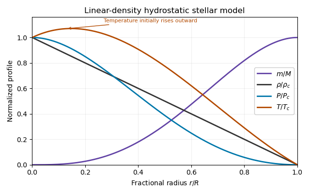
Write $\mathcal{R}=k/(\mu H)$, where $H$ is the atomic mass unit used in the mean molecular weight convention, and let $\kappa$ be the Rosseland mean opacity per unit mass. For a static spherical star with negligible thermal storage, the stellar structure equations areHere $ϵ$ is the net stellar energy-generation rate per unit mass; $a$ is the radiation energy-density constant and $c$ the speed of light. The last differential equation follows from radiative diffusion, $F=-(c/3\kappa \rho )d(a{T}^4)/dr$, with $L=4\pi r^{2}F$. There is no gravothermal storage term in the specified stellar energy balance equation. Neglecting radiation pressure in force balance does not remove radiation as an energy carrier. Regular central conditions are $m(0)=L(0)=0$; take negligible external pressure, $P(R)=0$, for the analytic hydrostatic equilibrium model below.

Set $x=r/R$. Integrating the enclosed mass directly givesThusThe stellar hydrostatic equation then givesFactorizing makes the surface behaviour transparent:The ideal gas equation of state gives the temperature profileNo small-$x$ approximation was needed. In particular, close to the centre,These exact hydrostatic formulas reveal a limitation of the prescribed linear-density stellar model. Its mass density has a central cusp, and $T^{\prime }(0^{+})=T_c/R>0$. A positive opacity with positive outward luminosity would instead require $T^{\prime }<0$ in radiative diffusion. Moreover, regular positive nuclear heating gives $L=O(r^3)$ and therefore $T^{\prime }=O(r)$ at the centre. Thus the imposed profile is a hydrostatic toy model, not a complete positive-heating radiative-equilibrium solution of all the stellar structure equations. The requested algebraic profiles and nuclear-luminosity integral can still be computed consistently as properties of that toy model.

Since $ϵ$ is per unit mass, each shell contributes $dL=ϵdm=4\pi r^2\rho ϵdr$. Both factors of mass density must be retained. Substituting the linear-density stellar model and its temperature profile givesWriting $I_{\nu }(z)$ for this incomplete integral, with $I_{\nu }=I_{\nu }(1)$, the luminosity isThis supplies both the local $L_r$ and the total luminosity associated with the printed integral extending to one. For fixed composition and fixed $\nu$, the total scales as $M^{2+\nu }{R}^{-3-\nu }$. The physical nuclear-heating exponents are positive; mathematically the surface integral converges for $\nu >-3$. As a simple normalization check, $I_0=1/30$, hence $L(R)=6{ϵ}_0{M}^2/(5\pi R^3)$ for temperature-independent heating. This is the generated luminosity; the radiative-transport incompatibility noted above is not removed by integrating the heating.

For a uniform-density stellar model, $\rho =3M/(4\pi R^3)$ and $m(r)=4\pi \rho r^3/3$. With zero surface pressure, integrate the stellar hydrostatic equation:Using the ideal gas equation of state, $T(r)=P(r)/(\mathcal{R}\rho )$. ThereforeEquivalently $P_c=3G{M}^2/(8\pi R^4)$ and $T_c=GM/(2\mathcal{R}R)$. The constant mass density is imposed as a structural approximation; a perfect gas can realize it hydrostatically by allowing its temperature and entropy to vary with radius.

For a stellar polytrope of index $n>0$, write $P=K{\rho }^{1+1/n}$ and combine hydrostatic equilibrium with mass conservation to obtainIntroduce Lane-Emden variables for a stellar polytrope, $\rho ={\rho }_c{\theta }^n$, $P=P_c{\theta }^{n+1}$ and $r=\alpha \xi$, whereSince ${\rho }^{-1}dP/dr=(n+1)P_c{\theta }^{\prime }/{\rho }_c\alpha$, the mechanical equation reduces to the Lane-Emden equationA constant-density interior corresponds to the formal polytrope of index zero, with $\rho ={\rho }_c{\theta }^0={\rho }_c$ where $\theta >0$. At $n=0$, regularity first gives ${\xi }^2{\theta }^{\prime }=-{\xi }^3/3$, and a second integration givesHere $P=P_c\theta =P_c(1-r^2/R^2)$ and ${\alpha }^2=P_c/(4\pi G{\rho }_c^2)$, reproducing $P_c=2\pi G{\rho }_c^2{R}^2/3$. The mass density jumps from its constant interior value to zero at the surface, while pressure vanishes continuously. The relation $P=K{\rho }^{1+1/n}$ is singular at $n=0$; the regular dimensionless pressure/mass density formulation defines this incompressible structural limit. It does not mean that the gas's perturbative stellar adiabatic exponent is infinite: the hydrostatic ideal-gas toy model and its adiabatic response are distinct choices.

The stellar adiabatic exponents are fixed-composition, constant-specific entropy derivatives:The chain rule gives ${\Gamma }_1({\Gamma }_2-1)/{\Gamma }_2={\Gamma }_3-1$. Define the pressure derivatives ${\chi }_{\rho }=(\partial \log P/\partial \log \rho {)}_T$ and ${\chi }_T=(\partial \log P/\partial \log T{)}_{\rho }$. The first law of thermodynamics, with $du=Tds+Pd\rho /{\rho }^2$, givesCombining this with $d\log P={\chi }_{\rho }d\log \rho +{\chi }_{T}d\log T$ on an adiabat givesThus the specific-heat ratio is not generally equal to the three stellar adiabatic exponents.

For the mixture, ${\chi }_{\rho }=\beta$ and ${\chi }_T=4-3\beta$. The specific heat capacity at constant volume, obtained by differentiating $u$ at fixed mass density, isTherefore the adiabatic exponents of a monatomic gas-radiation mixture and its specific-heat ratio areIf a relation involving only the exponents is wanted, eliminate $\beta$ from ${\Gamma }_1=\beta +(4-3\beta )({\Gamma }_3-1)$:For a pure monatomic perfect gas, $\beta =1$ and $\gamma ={\Gamma }_1={\Gamma }_2={\Gamma }_3=5/3$. For any calorically perfect gas with constant heat capacities, the same equality holds with its own ${\gamma }_g$. In a genuine gas-radiation mixture, $0<\beta <1$, $\gamma ={\Gamma }_1/\beta$ while the exponents are given separately above.

In the radiation limit, ${\Gamma }_1={\Gamma }_2={\Gamma }_3=4/3$ and the adiabatic temperature gradient is $1/4$. This follows independently from photon entropy: a comoving volume $V$ has $S\propto V{T}^3$, so an adiabat obeys $T\propto V^{-1/3}$ and $P\propto V^{-4/3}$. However, $c_P/c_V$ is singular in the pure-radiation limit, not $4/3$. This is the pure-radiation constant-pressure heat-capacity singularity. The equation $P=a{T}^4/3$ fixes temperature whenever pressure is fixed, so an ordinary constant-pressure temperature derivative is not available; along the mixture limit $\gamma \to \infty$ and $\beta \gamma \to 4/3$. For photons alone, mass-specific quantities additionally require a material mass label. The often quoted radiation index $4/3$ is its pressure-density adiabatic exponent, not a finite constant-pressure/constant-volume heat-capacity ratio.

Let $g=Gm/r^2>0$, $H_P=-dr/d\log P>0$, $\nabla =d\log T/d\log P$, and ${\nabla }_{\mu }=d\log \mu /d\log P$. Consider a small radial fluid displacement $\xi$ whose sound-crossing time is short enough to keep its pressure equal to its surroundings. Its composition is frozen and its heat exchange negligible. This is the local stellar convective stability test.

For gas-pressure-dominated ideal gas matter, $\rho \propto \mu P/T$. The ambient gradient is thereforeThe displaced element conserves specific entropy and mean molecular weight, giving $(d\log \rho /dr{)}_{\mathrm{parcel}}=-(1-{\nabla }_{\mathrm{ad}})/H_P$, where ${\nabla }_{\mathrm{ad}}=({\Gamma }_2-1)/{\Gamma }_2$. The parcel-minus-environment mass density difference isIts buoyancy acceleration is minus $g$ times this difference. ThusPositive stellar buoyancy frequency squared gives a restoring force. The gas-pressure-dominated Ledoux criterion is thereforeEquality is marginal in this ideal adiabatic test. For monatomic gas ${\nabla }_{\mathrm{ad}}=2/5$. An inward increase of mean molecular weight has ${\nabla }_{\mu }>0$ and stabilizes the layer; uniform composition recovers the Schwarzschild criterion. For a radiative layer one substitutes the stellar radiative temperature gradient, ${\nabla }_{\mathrm{rad}}=3\kappa LP/(16\pi acGm{T}^4)$.

More generally define $\delta =-(\partial \log \rho /\partial \log T{)}_{P,\mu }$ and $\phi =(\partial \log \rho /\partial \log \mu {)}_{P,T}$. The same displacement argument gives $N^2=(g/H_P)[\delta ({\nabla }_{\mathrm{ad}}-\nabla )+\phi {\nabla }_{\mu }]$ and stability for $\nabla <{\nabla }_{\mathrm{ad}}+(\phi /\delta ){\nabla }_{\mu }$. Both coefficients equal one in the gas-dominated ideal-gas limit used above. This is local dynamical stability against convection; it is distinct from global radial collapse and from instabilities requiring heat or composition diffusion.

Take a static, nonrotating, nonmagnetic spherical equilibrium with $\nabla P=-\rho \nabla \Phi$ and ${\nabla }^2\Phi =4\pi G\rho$. Use a fluid displacement $\mathbf{\xi }(\mathbf{r})e^{-i\omega t}$. Write $p_1,{\rho }_1,{\varphi }_1$ for Eulerian fluid perturbations. The Lagrangian pressure perturbation and corresponding mass density change obey $\Delta P=p_1+\mathbf{\xi }\cdot \nabla P$, $\Delta \rho ={\rho }_1+\mathbf{\xi }\cdot \nabla \rho$. Linearizing mass conservation, the Euler equations for an inviscid fluid and Poisson equation for Newtonian gravity givesThere is no equilibrium acceleration to multiply a perturbed mass density. The adiabatic process condition, with composition carried by the parcel, closes the system:These are the complete linear adiabatic stellar oscillation equations, including the perturbation of self-gravity. Neglect of heat exchange is appropriate when oscillation periods are short compared with relevant thermal relaxation times; it does not determine nonadiabatic excitation or damping.

For the pressure and buoyancy modes, separate angular dependence using spherical harmonics:The horizontal amplitude ${\xi }_h$ has dimensions of length. Angular differentiation gives $\nabla \cdot \mathbf{\xi }=[r^{-2}(r^2{\xi }_r{)}^{\prime }-\ell (\ell +1){\xi }_h/r]Y_{\ell }^m$, and tangential momentum gives ${\omega }^{2}r{\xi }_h=p_{\ell }/\rho +{\varphi }_{\ell }$. Define the adiabatic sound speed, stellar buoyancy frequency and Lamb frequency byThe adiabatic mass density relation becomes ${\rho }_{\ell }/\rho =p_{\ell }/(\rho c_s^2)+(N^2/g){\xi }_r$. Substitution produces a radial form of the full oscillation equations for nonzero $\omega$:The apparent $N^2/g$ factor is evaluated through its defining gradient at the centre rather than by dividing two zeros.

Regularity at the centre excludes singular solutions. At a free surface the Lagrangian pressure perturbation vanishes, $\Delta P=0$; outside the star the gravitational perturbation decays as $r^{-\ell -1}$. For a model with mass density tending to zero at its surface, continuity of ${\varphi }_{\ell }$ and its radial derivative gives ${\varphi }_{\ell }^{\prime }(R)=-(\ell +1){\varphi }_{\ell }(R)/R$. If the equilibrium mass density jumps to vacuum, include the displaced-surface mass sheet: the outward-minus-inward derivative jump is $4\pi G\rho (R){\xi }_r(R)$, so the interior condition is ${\varphi }_{\ell }^{\prime }(R)=-(\ell +1){\varphi }_{\ell }(R)/R-4\pi G\rho (R){\xi }_r(R)$. An atmospheric boundary condition can replace the ideal free surface.

These conditions make ${\omega }^2$ an eigenvalue, not an arbitrary local sound frequency. With conservative boundary conditions the adiabatic operator is self-adjoint, giving real ${\omega }^2$; negative values describe instability. The frequencies depend on $P(r),\rho (r),{\Gamma }_1(r)$, self-gravity, stratification and boundaries, as well as angular degree $\ell$ and radial order. In a spherical nonrotating star they are degenerate in $m$. For homologous equilibrium structures, their scale isthus the typical oscillation time measures inverse square root of mean mass density, while individual frequencies probe the interior adiabatic sound speed and stellar buoyancy frequency profiles.

For radial modes, write ${\xi }_r=r\eta$. Eliminating the pressure and gravitational perturbations gives the radial stellar pulsation equationThis is a Sturm-Liouville problem. Multiplication by $\eta$ and integration, with vanishing boundary terms, gives its Rayleigh quotientFor constant ${\Gamma }_1>4/3$, $P^{\prime }<0$ makes both numerator contributions nonnegative. At ${\Gamma }_1=4/3$, a homologous displacement is neutral; for constant ${\Gamma }_1<4/3$ the same trial displacement makes the quotient negative. For the uniform-density stellar model, $\eta =$ constant is an exact mode and ${\omega }^2=(3{\Gamma }_1-4)GM/R^3$. With varying ${\Gamma }_1$, the integral criterion, rather than a universal pointwise threshold, controls radial stability.

The Cowling approximation neglects ${\varphi }_{\ell }$ while retaining the equilibrium gravitational field. It is useful for short-wavelength modes, but is not needed for the full derivation above. In a locally slowly varying region, take both remaining amplitudes proportional to $e^{i\int k_{r}dr}$ and retain the leading derivative terms. ThenEliminating either amplitude gives the acoustic-gravity propagation relationPositive $k_r^2$ is oscillatory propagation; negative $k_r^2$ means an evanescent wave. The high-frequency branch, ${\omega }^2>S_{\ell }^2,N^2$, describes stellar acoustic modes, restored chiefly by compressibility and pressure. At frequencies well above $N$, this gives ${\omega }^2\simeq c_s^2[k_r^2+\ell (\ell +1)/r^2]$. The low-frequency propagating branch in stable stratification, ${\omega }^2<N^2,S_{\ell }^2$, instead describes stellar gravity modes, restored by buoyancy. At $\ell =0$ there is no such nonradial gravity-wave cavity.

A stellar acoustic mode is trapped between an inner turning point near $\omega =S_{\ell }$ and an outer reflecting region. Low-$\ell$ modes penetrate deeply; radial modes reach the centre. Higher-degree modes turn farther out. Standing waves require the WKB quantization conditionwhere the phase $\alpha$ depends on the central or turning-point behaviour and surface reflection. For high radial order and small degree, the leading acoustic travel-time result is the large frequency separationThe $\ell /2$ term is the leading central angular phase shift; smaller frequency separations depend on detailed interior gradients. The near-surface mass density stratification sets the acoustic cutoff frequency. In a plane-parallel isothermal atmosphere with mass density scale height $H_{\rho }$, ${\omega }_{\mathrm{ac}}\simeq c_s/(2H_{\rho })$. Modes below this cutoff can reflect and form a cavity; waves sufficiently above it escape and need an outgoing-wave boundary condition. Nonadiabatic damping, driving and rotation alter real-star mode properties, but the adiabatic frequency problem isolates their dependence on the equilibrium structure.