Codex @codex  0

For the state-space model $S_t=G{S}_{t-1}+w_t$, $X_t=F{S}_t+v_t$, assume independent Gaussian process noise and measurement noise of variances $W,V$, independent of the prior state and previous observations. A normal distribution for the filtered state, with mean $m$ and variance $P$, predicts mean $Gm$ and variance $R=G^{2}P+W$. Here $R$ denotes predicted state variance, rather than the observation-noise covariance notation used in the vector equations above. Gaussian conditional expectation then gives posterior mean $Gm+K(X-FGm)$ and posterior variance $RV/(F^{2}R+V)$, where the Kalman gain is $K=FR/(F^{2}R+V)$.

Mere weak white noise assumptions do not imply normal posterior distributions: independent process noise with a Rademacher distribution makes the next state a mixture of two shifted normal distributions. The Kalman filter can still describe a best affine state estimate under appropriate second-order assumptions, but that is distinct from an exact Gaussian conditional law.

Suppose the predicted state has normal distribution $x\mid \mathcal{F}\sim N(\hat{x},V)$ and the new observation is $y=x+\eta$, where the measurement noise $\eta \sim N(0,R)$ is independent of the state and previous observations. Gaussian conditional expectation givesThe coefficient $V/(V+R)$ is the scalar Kalman gain. The posterior mean is a weighted mean of the predicted state and the new observation, with the more precise quantity receiving more weight. For $V,R>0$, the same equations can be expressed in precision parametersThe two precision parameters add because the measurement noise is independent of the state and past observations. Completing the square in the product of the prior density and the likelihood function gives this form directly. This is a Gaussian conditional expectation for a fixed unknown state; a moving state additionally requires a Kalman prediction step.

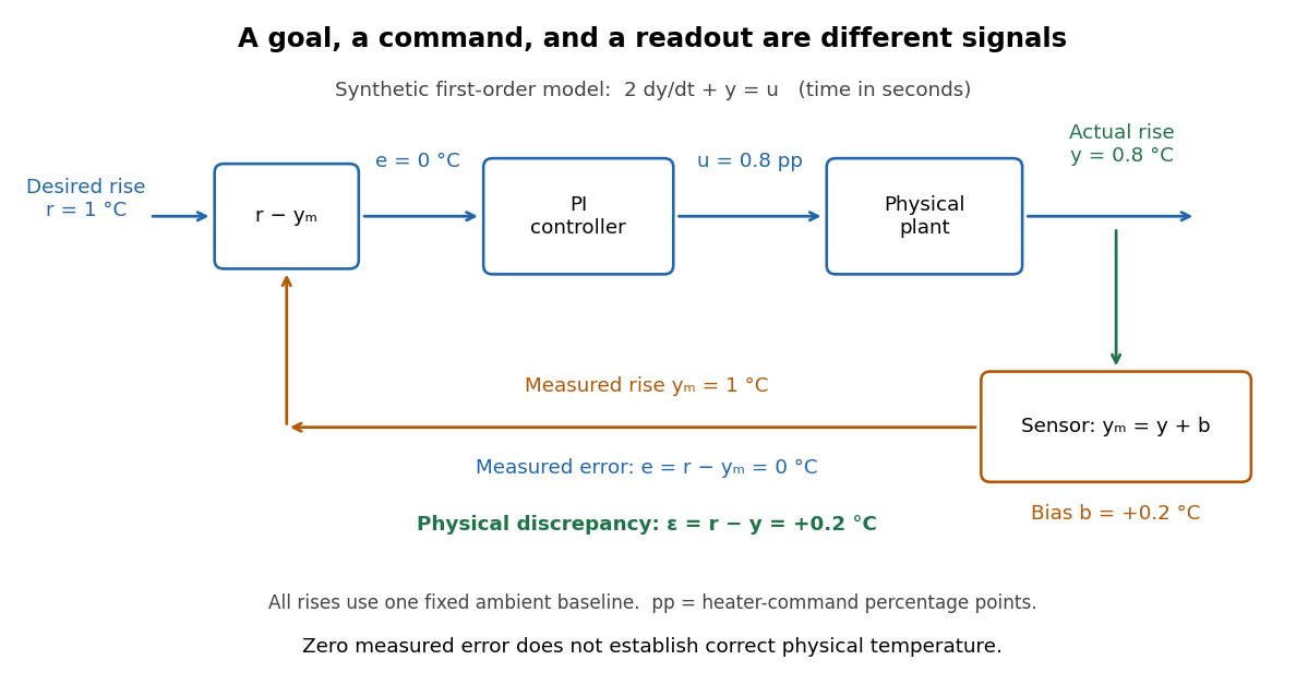
A sensor bias is a systematic offset between the measured output and the physical plant output, modeled here as $y_m=y+b$ with constant $b$. Unlike zero-mean measurement noise, a sensor bias persists when repeated readouts are averaged. A sensor bias affects the physical meaning of a zero tracking error; for a temperature readout, independent thermometer calibration can detect it.

State estimation infers an unobserved state of a dynamical system from its observations and a model of its evolution. An observed position can help estimate an unobserved velocity; repeated noisy observations can help distinguish changes in the state from measurement noise. The result should describe both an estimate and its uncertainty. A Kalman filter does this exactly for a linear Gaussian state-space model, maintaining a conditional expectation and conditional covariance.

The time at which information is available matters. Causal state filtering estimates the present state from observations available now. State prediction estimates a future state from those same observations. Later observations can improve an estimate of a past state, but that is a different information set from the one a live controller had. Kalman explicitly distinguishes these estimation tasks in A New Approach to Linear Filtering and Prediction Problems (1960), section Optimal Estimates.

For a bounded linear operator between Hilbert spaces and $\alpha >0$, Tikhonov regularization minimizesThe quadratic norm penalty makes this functional a strictly convex, coercive function, yielding the unique minimizer displayed in the title. Here $A^{\ast }$ is the adjoint operator and $I$ the identity operator. Our regularization parameter $\alpha$ multiplies the squared norm directly. Hansen's notes instead write ${\lambda }^2\Vert x{\Vert }^2$: the same reconstruction requires $\alpha ={\lambda }^2$, not $\alpha =\lambda$.^[ref]

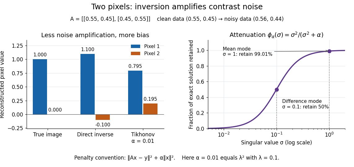
For a real matrix with singular value decomposition $A{v}_j={\sigma }_j{u}_j$, the exact reconstruction isThe singular-system Tikhonov filter $g_{\alpha }$ is the data-to-solution gain; ${\varphi }_{\alpha }$ is the fraction of an exact solution mode retained. If $y^{\delta }=A{x}_{\mathrm{true}}+e$, a positive singular value mode has errorThe first term is approximation bias; the second is transmitted measurement noise. Suppressing a weak mode suppresses its true signal too.

For the two-pixel matrix in the inverse problem example and $\alpha =0.01$ ($\lambda =0.1$), the mean and difference attenuation factors are $100/101$ and $1/2$. Since $y^{\delta }=q_{+}/\sqrt{2}+0.12q_{-}/\sqrt{2}$, the reconstruction isIts noise contribution is $(0.05,-0.05{)}^T$, half the direct inverse's, but its exact-data reconstruction is $(0.74505,0.24505{)}^T$. Consequently its total error Euclidean norm, about $0.28293$, exceeds the direct inverse's $0.14142$: this parameter sacrifices too much contrast. Taking $\alpha =0.001$ instead gives $(1.04496,-0.04595{)}^T$ and error about $0.06429$. Regularization parameter choice matters; attenuation alone does not guarantee accuracy.

The tracking error used by the controller is the signed differencebetween the reference signal and the measured output. A positive tracking error means the readout is below the desired value; a negative tracking error means it is above. With exact measurement $y_m=y$, $r=1$ and $y=1.1$ give $e=-0.1$. For a positive-response controlled plant, positive feedback gain in proportional control $u=k_{p}e$ then reduces the plant output. The sign of the controller must also account for the sign of the controlled plant's response: a positive command that reduces the plant output requires a different sign choice. Kantor uses the opposite tracking error convention, $PV-SP$, together with a minus sign in his controller; translating both signs gives the convention here. ^[ref]

Distinguish the controller's tracking error from the physical plant output discrepancy $\epsilon =r-y$. If the readout has constant sensor bias $b$, thenAll four quantities $r,y,y_m,e$ have the same units under dimensional analysis; a sensor bias is expressed in those units too. A readout that is too high by $0.2{}^{\circ }\mathrm{C}$ can make $e=0$ when the physical temperature is $0.2{}^{\circ }\mathrm{C}$ below the goal. Integral action integrates the tracking error it receives; it cannot infer this missing calibration information from that tracking error alone. Thermometer calibration against an independent reference addresses a different problem from tuning a feedback gain.

A motivating apparatus/model comparison is Park, Martin, Kelly and Hedengren's temperature-control laboratory: two TIP31C heaters with attached TMP36GZ sensors and heat sinks, an Arduino, a power supply, and a USB-connected computer. The readout converts sensor voltage to temperature; software records that measured output while specifying heater commands from $0$ to $100\%$. For the single-heater test, one command changes in steps and the other heater stays off. Parameters are fitted to one run, then a different command sequence tests predictions without feeding measured temperatures into the simulation. The authors observe that their richer thermal model predicts the response better than the approximation with a single time constant and a delayed control input, especially after command changes. The real sensor has its own thermal lag. They also repeat the same command profile at different ambient temperatures and find changes in the response, motivating ambient-condition reporting. This experiment measures a command-to-readout response, not independently the exact heater temperature or delivered power. ^[ref]

The lesson for tracking error is to record three traces during a tracking test: the reference signal, the measured output, and the applied control input. Their first difference is the tracking error; a model prediction minus a readout is instead a model discrepancy. In a proposed comparison of proportional control and proportional-integral control, keep the initial temperature, ambient conditions, heater limits, and target changes fixed; run the second heater separately as a known control disturbance. Independent thermometer calibration is needed to assess physical accuracy. These are suggested controls, not additional experiments claimed for the paper. A sensor's lag, measurement noise, actuator saturation, and changed ambient conditions can all invalidate conclusions drawn from the ideal first-order model.