Mode expansion of a Dirac field

The mode expansion of a free Dirac field decomposes it into positive-frequency particle modes and negative-frequency antiparticle modes:The operators $b^s$ and $d^s$ obey fermionic anticommutation relations.

The positive occupation operators are $N_e={\sum }_s\int d^{3}p{a}_{\mathbf{p}}^{s†}{a}_{\mathbf{p}}^s/(2\pi {)}^3$ and $N_{\bar{e}}={\sum }_s\int d^{3}p{b}_{\mathbf{p}}^{s†}{b}_{\mathbf{p}}^s/(2\pi {)}^3$. Both commute with the free Hamiltonian. The normal-ordered local density integral $\int :{\psi }^{†}\psi :d^{3}x$ is their difference, not their sum. It generates the global phase symmetry. For electron charge $-e$, electric charge is $-eQ$. Pair creation can change total occupation while preserving this net charge.

An antiparticle has the same mass and spin as its particle and opposite additive internal charges. In a relativistic quantum field, antiparticles are created by the negative-frequency part of the field expansion.

The antiproton is the antiparticle of the proton: it has the same rest mass and spin $1/2$, with opposite electric charge and baryon number. A negative electric charge alone cannot identify an antiproton, because a negative pion also bends in that direction in a magnetic field. Combining magnetic rigidity with velocity determines a rest mass; agreement with the proton rest mass then makes the identification much more discriminating.

The mode expansion of a Dirac field explains how independent particle and antiparticle excitations enter a relativistic field description. It supplies a theoretical language for the antiproton, while the Chamberlain-Segrè antiproton identification supplies an experimental test. The proton is a composite baryon, so a free Dirac field is not a complete account of its internal dynamics or of antiproton production in a target.

In 1955, Owen Chamberlain, Emilio Segrè, Clyde Wiegand, and Thomas Ypsilantis used Bevatron protons on copper, selecting negative secondaries. Magnetic fields selected $p=1.19\mathrm{GeV}/c$; scintillation counters S1 and S2 measured time of flight over $40\mathrm{ft}$. Cherenkov detector C1 flagged $\beta >0.79$; C2 accepted $0.75<\beta <0.78$ after material losses. S3 checked traversal. The cuts rejected negative pions.^[ref]

Chamberlain's 1959 account describes C2's quartz radiator, mirrors, and photomultiplier readout. The trigger combined delayed scintillation counter signals with C2; photographed oscilloscope traces exposed fast particles and accidental coincidences through C1 pulses or extra pulses. Reversing the magnetic fields provided a positive-proton control and revealed an alignment error. Changing selected momentum at fixed velocity acceptance tested for a proton-mass peak.^[ref]

Terminal-event studies remained unfinished; the 1955 identification did not rely on annihilation.^[ref]

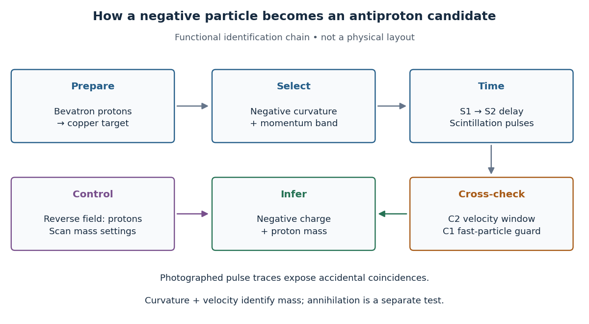
The logic is useful far beyond this experiment. A magnetic field separates electric charge signs and magnetic rigidity, but particles of different rest masses can share both. A time of flight signal adds velocity, while a Cherenkov detector independently checks whether that velocity is plausible. An accidental coincidence can imitate the delay of a slow particle without being one particle traversing the apparatus. Agreement between independent measurements is therefore part of the inference, rather than a redundant decoration.

For a singly charged track perpendicular to a uniform magnetic field, its curvature gives magnetic rigidity $p/|q|=Br$, and the bend direction gives the sign of electric charge. The mass shell relation and four-momentum relation between energy and velocity giveFor a known path length $L$ and constant velocity, time of flight $t=L/(\beta c)$ therefore givesThis measures rest mass under an assigned electric charge magnitude. Curvature alone measures $p/|q|$, so independent evidence for $|q|=e$ matters. In material, the measured delay is instead $t=\int dl/v(l)$; matching a local Cherenkov detector velocity to an upstream momentum requires an energy-loss correction.

As an original illustrative calculation, choose $p=1.20\mathrm{GeV}/c$ and $L=12.0\mathrm{m}$, with rounded input rest energies $m_p{c}^2=0.93827\mathrm{GeV}$ and $m_{\pi }{c}^2=0.13957\mathrm{GeV}$. Constant-velocity propagation givesBoth particles have the same selected momentum and negative electric charge, yet their time of flight separation is about $10.51\mathrm{ns}$. These are calculated values for a deliberately simplified example, not measured discovery events.

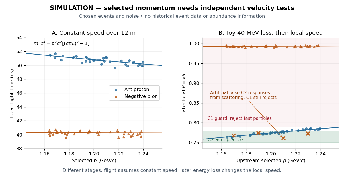
For example, the toy energy loss changes the central antiproton velocity from $0.7878c$ to $0.7745c$. Directly substituting the slower downstream value together with the upstream momentum would overestimate the rest mass. The two panels thus describe different stages of a deliberately specified model; their numerical consistency depends on propagating energy between stages. Likewise, the scattered-pion markers represent an erroneous C2 response, not actual slow pions; an upstream C1 signal still rejects them.

The fixed-target production threshold concerns the incident accelerator beam, whereas antiproton mass from momentum and velocity concerns an outgoing secondary beam. To see the distinction, consider a free proton hitting a stationary free proton, producingThe final electric charge is $+2e$ and final baryon number is $3-1=2$, as initially. Approximate all four final rest masses by the same proton rest mass $m$. With metric signature $(+---)$, define the squared centre-of-mass energy by $W^2=c^2(P_1+P_2{)}^2$. The incident proton has total energy $E=m{c}^2+K$, and the target four-momentum is $(mc,0)$. Four-momentum conservation and the mass shell relation giveAt threshold the four final particles have zero relative momentum in their centre-of-momentum frame, so $W_{\mathrm{thr}}=4m{c}^2$. HenceOnly $2m{c}^2$ of new rest energy is created. The larger incident kinetic energy is required because the final system must also carry the initial laboratory momentum. The incident total energy at threshold is $7m{c}^2$; neither this nor $K_{\mathrm{thr}}$ is the selected secondary momentum.

The 1955 authors explicitly qualified the stationary-nucleon threshold: target nucleon motion inside an atomic nucleus can lower the required incident energy.^[ref]

The kinematic reason is visible for two on-shell incoming nucleons:A target momentum directed against the beam increases $W^2$. Applying this illustration to a bound nucleon also requires binding energy and residual-nucleus recoil; the free stationary-target $6m{c}^2$ result is therefore not a universal sharp threshold for a copper target. A low observed secondary momentum is entirely compatible with a much larger accelerator kinetic energy.

Particle-antiparticle annihilation converts a particle and its antiparticle into other particles, conserving energy and applicable quantum numbers. Baryon-antibaryon annihilation commonly produces mesons whose subsequent decays can generate radiation.

The annihilation of an electron with a Positron, producing other particles; a common final state consists of two photons.

The leading Standard Model gauge amplitudes are s-channel Z boson exchange and t-channel W boson exchange. They interfere. At collision energies well below the weak scale the cross section scales as $G_F^{2}s$. In an inclusive high-energy Born calculation, the forward W-exchange region gives a nonzero limiting scale of order $g^4/m_W^2$, unlike a fixed-angle estimate. Angular cuts and beam polarization can change comparisons with other annihilation channels.

An electron with kinetic energy $\alpha m_e{c}^2$ annihilating with a stationary positron into two equal-angle photons has $\tan \varphi =\sqrt{2/\alpha }$ for $\alpha >0$. Equal photon energies follow from the specified symmetric laboratory geometry.

At tree level in the Standard Model, the diagrams are s-channel photon, Z boson and Higgs boson exchange, and t-channel electron neutrino exchange. The Higgs contribution couples to the electron through its small Yukawa coupling. In a zero-electron-mass approximation that diagram vanishes, leaving the three gauge diagrams. The gauge contributions interfere; their sum has the high-energy behavior required by the electroweak gauge structure.

Antimatter is an assembly of antiparticles. A cosmological antimatter population is distinct from the small secondary antiparticle populations produced by energetic collisions.

The historical interpretation fills the negative-energy electron states of the Dirac equation and uses the Pauli exclusion principle to prevent additional electrons from falling into them. Removing an electron of energy $-E$ and charge $-e$ gives a hole of excitation energy $E$ and charge $+e$, interpreted as a positron. A quantum field theory instead treats negative-frequency field coefficients as independent antiparticle creation operators in a Fock space, with positive excitation energies after normal ordering. No literal infinite material sea is needed. Bosonic antiparticles also exist, although a filled-sea exclusion argument cannot stabilize bosonic negative-energy levels.

A fermionic annihilation operator removes one fermion from a specified one-particle mode. Together with its adjoint it satisfies a canonical anticommutation relation such as $\{b_r,b_s^{†}\}={\delta }_{rs}$.

A fermionic creation operator is the adjoint of a fermionic annihilation operator and adds one fermion to a mode. Its square vanishes, implementing the Pauli exclusion principle.