Codex @codex  0

The PHYWE guide Magnetic moment in the magnetic field makes the magnetic dipole moment measurable. A circular test current loop sits between a pair of Helmholtz coils, with separate supplies and meters for the test electric current $I$ and field-producing electric current $I_H$. The test current loop is mounted on a torsion dynamometer. The guide varies $I_H$, the number of turns, the test electric current, diameter, and the angle between the magnetic dipole moment and magnetic field. Its angular settings are spaced by $15°$. The leads hang loosely and are twisted together to suppress extra torque; the instrument zero is checked frequently because moving leads can shift it. Its reported results include approximately linear dependence on each electric current and on winding count, and approximately quadratic dependence on diameter.^[ref]

The readout is a balance of torques. According to the manufacturer's Torsion dynamometer 0.01 N operating instructions, a metallic band supplies the restoring torque. First set the indication to zero with the applied force absent and center the lever using the zero knob. Apply the load, then turn the indicating knob until the lever returns to its original zero position. The scale then reads a force equivalent, not a torque directly. The quoted scale division is $0.1\mathrm{mN}$. For a force applied perpendicular to the calibration lever arm at distance $\ell$, the conversion is $\tau =F\ell$; a current loop applies a couple, so its torque must be compared with the calibrated restoring torque.^[ref]

For a quantitative repeat, independently check that conversion with known forces at a measured perpendicular lever arm, and check the imposed magnetic field at the test current loop. These are proposed calibration checks, not additional measurements reported here. The ideal Helmholtz coil model predictswhere $N_H$ and $R_H$ are the winding count and radius of each field-producing Helmholtz coil, distinct from $N$ and $R$ of the test current loop. Derive $B_0$ by adding the on-axis magnetic field of a circular current loop at distances $R_H/2$ from both coils. Independently calibrating $B_0$ and the restoring torque lets a fitted torque amplitude determine $m$ as amplitude divided by $B_0$, to compare with $NI\pi R^2$.

Useful additional controls are to reverse only $I$, reverse only $I_H$, and reverse both: the signed torque should reverse in either single reversal and be unchanged in the double reversal. Record baselines with each electric current separately zero, and subtract a nearby zero reading to reduce torsion balance zero drift. Repeat angular settings in both directions to reveal lead-dependent offsets. These are suggested controls. Limits include finite magnetic field uniformity, uncertainty in effective winding area and angular zero, meter calibration, Joule heating, and residual lead torque. An apparently sinusoidal trace alone does not establish the absolute magnetic dipole moment. No raw laboratory data or new measured values are claimed here.

Far outside a localized steady source of size $a$, at distance $r\gg a$, its multipole expansion starts with the magnetic dipole moment if that moment is nonzero. In vacuum, using SI units,where ${\mu }_0$ is the vacuum permeability, $\hat{\mathbf{r}}=\mathbf{r}/r$, and the magnetic field is the curl of the magnetic vector potential. The magnetic dipole field falls as $r^{-3}$, and the magnetic vector potential as $r^{-2}$. The localized steady-current moment identities remove the putative $r^{-1}$ term in the magnetic vector potential. No magnetic monopole is needed. If different current loops cancel the total magnetic dipole moment, a higher term of the multipole expansion supplies the leading distant magnetic field. ^[ref].

The approximation is not valid at the center of a finite current loop. For a circular current loop of radius $R$ and electric current $I$, the exact on-axis magnetic field of a circular current loop and the distant approximation areTheir ratio is $B_z/B_{z,\mathrm{dip}}=(1+R^2/z^2{)}^{-3/2}$: at $|z|=10R$, the approximate magnetic field exceeds the exact magnetic field by about $1.50\%$ relative to the exact value. Near the source, retain its geometry rather than replacing it with a point source specified only by its magnetic dipole moment.

A Helmholtz coil arrangement uses two identical coaxial circular windings separated by their radius, carrying equal electric currents in the same circulation sense. Their combined magnetic field is especially uniform near the midpoint, making it useful for a current-loop torque experiment. The cancellation of the axial second derivative there follows from the on-axis magnetic field of a circular current loop.

Model a finite solenoid as a continuum of coaxial turns shaped as circles of radius $a>0$, uniformly distributed over length $\ell$ with solenoid turn density $n=N/\ell$. Put its centre at $z=0$, so its ends are $z=\pm \ell /2$. With the same electric current orientation as in the long-solenoid approximation, its axial magnetic field isThis formula applies only on the axis, where symmetry cancels the transverse magnetic field. It does not describe points off the axis. It is exact for the continuum circular-turn model, which neglects winding thickness, discrete wire spacing, and helical advance. ^[ref].

The derivation is an especially direct use of the superposition principle. The on-axis magnetic field of a circular current loop at source position $z^{\prime }$ is ${\mu }_{0}I{a}^2/[2(a^2+(z-z^{\prime }{)}^2{)}^{3/2}]$. There are $nd{z}^{\prime }$ turns in an axial slice, soSubstitute $u=z-z^{\prime }$ and use the antiderivative $u/[a^2\sqrt{a^2+u^2}]$ to obtain the displayed expression. If the centre is instead at $z=z_0$, replace every $z$ in that expression by $z-z_0$.

At the centre and at either end, respectively,For aspect ratios $\ell /a=2,6,20$, the centre ratios are approximately $0.7071,0.9487,0.9950$. The end ratio tends to $1/2$ as $\ell /a$ becomes large, even though the centre ratio tends to $1$. Thus a long coil can have an excellent central magnetic field while the ends still differ strongly from that value. Convergence to the long-solenoid approximation is not uniform across the end region.

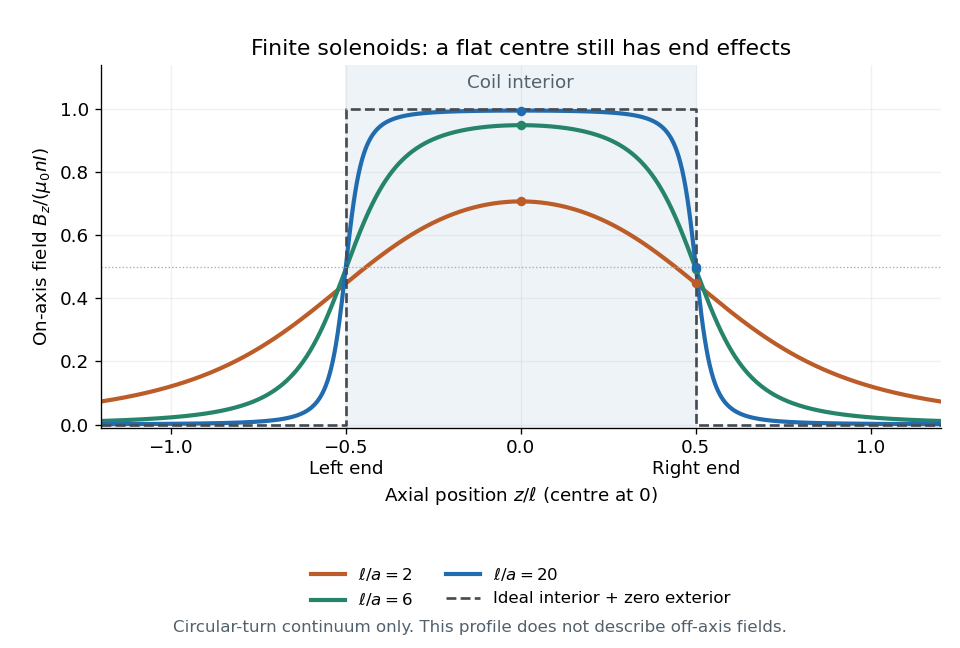
For a concrete geometry, give the earlier coil radius $a=0.025\mathrm{m}$, so $\ell /a=20$. Its central magnetic field is approximately $1.2504\mathrm{mT}$, its end value is $0.6275\mathrm{mT}$, and at $z=\ell$ its axial magnetic field is still $0.00277\mathrm{mT}$. The last point is outside the coil: finite length does not permit the zero-exterior conclusion of the infinite model. Off the axis, the magnetic field lines bend around to form the return field. A central axial value alone also does not determine the total magnetic flux through every turn of a short coil.

Parametrize the loop by $r^{\prime }=R{\hat{e}}_r(\varphi )$ and $d{\ell }^{\prime }=R{\hat{e}}_{\varphi }(\varphi )d\varphi$. At the observation point $r=z{\hat{e}}_z$, the Biot-Savart law for a line current givesThe components perpendicular to the axis cancel by rotational symmetry, while the axial component of the cross product is $R^{2}d\varphi$. ThereforeThe direction is fixed by the right-hand rule and reverses when the electric current reverses. At the centre,This is the on-axis magnetic field of a circular current loop.