Past exam of the advanced fluid dynamics course of the University of Oxford / 2024 / 1

Start in an inertial frame with the inviscid magnetohydrodynamic momentum equation,Here $\rho$ is mass density, $P$ is the isotropic fluid pressure, $\mathbf{v}$ is inertial-frame velocity, $\mathbf{J}$ is electric current density, $\mathbf{B}$ is the magnetic field, and $\Phi$ is gravitational potential per unit mass. In the low-frequency approximation to Ampère's law, $\mathbf{J}=\nabla \times \mathbf{B}/{\mu }_0$. The vector calculus identityseparates the Lorentz force density into magnetic tension and a magnetic pressure gradient. Transform the material acceleration to a rigid frame rotating with constant angular velocity ${\mathbf{\Omega }}_0$, using the stated frame transformation. The rotating-frame magnetohydrodynamic momentum equation isThe final terms are the Coriolis force and centrifugal force densities; $\mathbf{u}$ is the velocity relative to the rotating frame, and $D_t={\partial }_t+\mathbf{u}\cdot \nabla$ uses that frame.

This requires a smooth conducting-fluid continuum with nonrelativistic motion, a constant magnetic permeability ${\mu }_0$, the solenoidal magnetic-field constraint, a negligible displacement current and negligible net electric-charge force. Viscous forces and anisotropic fluid stresses are omitted. A time-dependent frame would add an Euler force. Incompressible flow is not needed for this force equation. Finite electrical resistivity does not change its displayed instantaneous magnetic force; the later frozen-field calculation additionally uses ideal magnetohydrodynamics. A differentially rotating fluid does not define a single rigid frame with spatially varying ${\mathbf{\Omega }}_0$: choose a fixed local reference rate and retain the fluid's shear in $\mathbf{u}$.

In an inertial frame, a circular orbit at radius $R$ has radial acceleration $-R\Omega (R{)}^2{\mathbf{e}}_R$. Neglecting fluid and magnetic forces givesIn a local rotating frame with ${\Omega }_0=\Omega (R_0)$, the fluid is instantaneously at rest at the reference radius $R_0$. The radial centrifugal force $+\rho R_0{\Omega }_0^2$ then balances the inward gravitational force. Away from $R_0$, the fluid's nonzero rotating-frame velocity must also be retained; the entire differentially rotating disk is not at rest in that one frame.

Take outward radial force as positive and keep the displaced element's angular rate fixed at ${\Omega }_0=\Omega (R_0)$. Its imbalance isUse the equilibrium relation from part b, ${\Phi }^{\prime }(R)=R\Omega (R{)}^2$, and a first-order Taylor expansion:The absolute values are needed for a magnitude. As printed, the proposed magnitude has a signed right side; it would be negative for outward displacement in a Keplerian disk. For decreasing ${\Omega }^2$, the signed imbalance above points outward and therefore amplifies that fixed-angular-rate displacement. This calculation fixes the angular rate, rather than the specific angular momentum; the latter is the conserved quantity for an uncoupled inviscid radial displacement and leads to the Rayleigh centrifugal stability criterion.

Linearized magnetic flux freezing gives the Eulerian magnetic field perturbationThe background is uniform, and incompressibility gives $\nabla \cdot \mathbf{\xi }=0$. For a horizontal displacement proportional to $e^{ikz}$, $\delta \mathbf{B}=ik{B}_0\mathbf{\xi }$ and $\delta B_z=0$. Thus the first-order magnetic pressure perturbation vanishes, and the magnetic-tension response to an incompressible displacement isBending a field line produces a restoring force proportional to displacement, like a spring obeying Hooke's law. Per unit mass, its squared spring frequency is $k^2{v}_A^2$, where $v_A=B_0/\sqrt{{\mu }_0\rho }$ is the Alfvén speed. The equilibrium can be independent of $z$ while the perturbation varies with $z$; neglect of background vertical structure does not set this perturbation's wavenumber to zero.

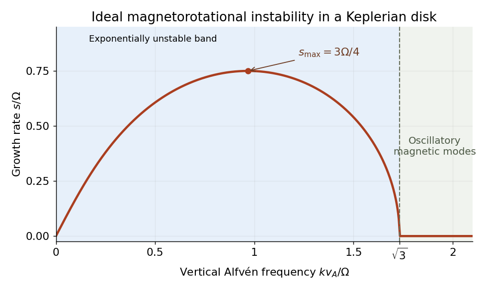
Work locally at $R_0$ with $\Omega =\Omega (R_0)$, and defineHere $\kappa$ is the radial epicyclic frequency. Combining the radial imbalance, the Coriolis force and the magnetic spring gives the spring model of magnetorotational instability:For a normal mode proportional to $e^{-i\omega t}$, the coefficient matrix isSetting its determinant to zero yields the ideal magnetorotational dispersion relation,Its two values of ${\omega }^2$ areso they are real. For $a>0$, their product is negative exactly when $a+D<0$, giving an exponentially growing normal mode. Conversely, $a+D>0$ also makes their sum positive and therefore gives two positive squared frequencies. A fixed nonzero magnetic mode is exponentially unstable for $k^2{v}_A^2+D<0$, oscillatory for $k^2{v}_A^2+D>0$, and marginal at equality. Stability against every allowed nonzero wavenumber in the unbounded ideal model requires $D\ge 0$; finite-domain restrictions can remove the unstable band.

For $\Phi =-GM/R$, the equilibrium relation gives ${\Omega }^2=GM/R^3$, so $D=-3{\Omega }^2$ and ${\kappa }^2={\Omega }^2$. Hence the Keplerian disk has the magnetorotational instability bandWithout the magnetic field, the polynomial becomes ${\omega }^2({\omega }^2-{\kappa }^2)=0$. The Rayleigh centrifugal stability criterion instead requires ${\kappa }^2>0$, equivalently $d(R^4{\Omega }^2)/dR>0$. A Keplerian disk satisfies that hydrodynamic criterion. Magnetic coupling therefore destabilizes a disk that has a restoring hydrodynamic epicyclic oscillation; the field couples angular-momentum exchange between elements, rather than acting only as an isolated restoring spring.

The plotted maximum is the maximum growth rate of ideal magnetorotational instability, $3\Omega /4$ at $k^2{v}_A^2=15{\Omega }^2/16$.