Source: released examination bundle,
Part A 2007 11-1.pdf, pages 121–124. All nine questions are covered. No mark allocations are printed.The zero polynomial belongs to . If , linearity gives . If and , polynomial evaluation obeys , so . Thus is an ideal of the polynomial ring .
The vectors are linearly dependent in the -dimensional vector space. Their dependence supplies a nonzero polynomial of degree at most in . Hence this ideal is nonzero. A polynomial ring over a field is a Euclidean domain under degree, and every ideal in a Euclidean domain is principal. It follows that for a nonzero polynomial , which can be scaled uniquely to be monic.
For completeness, uniqueness follows because any two generators divide each other and hence differ by a nonzero constant; the monic normalization forces that constant to be one. Since divides the polynomial of degree at most constructed above, its degree is at most . The generator characterization givesThis is the minimal polynomial of a vector under a linear operator. If , the ideal is the whole ring and the unique monic generator is the constant polynomial one.
A self-adjoint operator satisfies for every . The finite-dimensional finite-dimensional spectral theorem gives an orthonormal basis of eigenvectors and real eigenvalues; eigenvectors for distinct eigenvalues are orthogonal. Consequently a matrix represents a self-adjoint transformation in some, possibly nonorthonormal, basis exactly when it is diagonalizable with real eigenvalues.
For , the eigenvalues are , all distinct and real. Eigenvectors are , , and . Thus can represent a self-adjoint transformation after choosing a suitable basis.
For , the eigenvalue one has algebraic multiplicity two but its eigenspace has dimension one. The lower block is a nontrivial Jordan block, so the matrix is not diagonalizable. Hence cannot represent a self-adjoint transformation in any basis.
For , the eigenspace for two is spanned by and , and the eigenvalue-one eigenspace is spanned by . These three vectors form an eigenbasis. Therefore can represent a self-adjoint transformation. To see sufficiency on the given inner product space, first define the real diagonal transformation in an orthonormal basis and then apply the inverse of a diagonalizing basis change to obtain the requested matrix. Symmetry of the displayed matrix itself would be required only for an orthonormal representing basis.
A cubic over a field is reducible exactly when it has a root in that field. For modulo five, direct evaluation givesNo value is zero, so is irreducible in .
The integer polynomial in the second part reduces to precisely , because , and . It is monic, hence primitive, and its degree is preserved by reduction. The irreducibility by degree-preserving reduction modulo a prime criterion states that a primitive integer polynomial with irreducible reduction of the same degree is irreducible over the rationals. This follows from Gauss's lemma: a rational factorization would give integer factors whose leading coefficients remain nonzero modulo five, contradicting the irreducible reduction. Thus
For closed sets in , the answers are : no; : yes; : yes. The first interval omits its limit point zero. The second contains its finite limit points, and the empty set is closed in every topology.
For open sets in , the answers are : yes; : no; : yes. Every point of the positive ray has a small interval contained in it, while zero is not an interior point of the nonnegative ray. The empty set is open by the topology axioms.
For open sets in , the answers are : no; : no; : yes. Every complex disk centered at a real point contains nonreal points, so a nonempty subset of the real axis cannot be open in the complex plane. The empty set remains open.
The modulus map is continuous, the denominator is positive everywhere, and sums, products and quotients with nonzero denominator preserve continuity. Hence is continuous throughout .
For , , so as . The chosen argument is continuous locally away from the negative real axis, making continuous there as well. At a point , , approach along . From , ; from , . The value assigned on the cut is . Thus is discontinuous at every strictly negative real point, and therefore is not a continuous map on the entire complex plane. Its radial factor is , as printed, rather than the of a square root.
For , the Cauchy-Riemann equations are and . Holomorphy implies these relations. Conversely, if the first partial derivatives exist and are continuous near a point, satisfying the equations there gives complex differentiability; satisfying them on an open set gives a holomorphic function on that set.
Let . On the cut plane, : equality could occur only at a nonpositive real point, which is excluded. Thus is strictly positive and is well defined and smooth. Since ,ConsequentlyOne can verify holomorphy directly:Here throughout the domain, so all partial derivatives are continuous. Therefore is holomorphic, specifically the principal square root on the cut plane, with derivative .
The two bounding circles meet at zero and one, which the Möbius transformation sends to zero and infinity. They therefore become straight lines through zero. More explicitly write , so . The two disk inequalities becomeSince , these say . ThusThe positive real axis belongs to the image because , fixing which sector is intended. Cubing maps this sector bijectively onto the right half-plane: its argument interval of width becomes . The Cayley transform between the half-plane and disk then maps that half-plane bijectively onto the unit disk. Hence a holomorphic bijection isEvery denominator is nonzero on the corresponding domain, and the sector width ensures the power map is injective. This is the conformal map of a symmetric circular lens.
If two solutions exist, their difference satisfies with , where . The general solution is . The first endpoint gives and the second gives , hence . Thus the solution is unique if it exists.
For the operator , choose the homogeneous solutions and satisfying the left and right endpoint conditions. Continuity at and derivative jump yield the Dirichlet Green functionIndeed it vanishes at both endpoints and satisfies . Splitting the integral at and differentiating verifies that is twice continuously differentiable for continuous and solves the boundary-value problem, establishing existence as well.
The characteristic equations for a transport equation are , , . Label an initial point by and choose characteristic time zero on the data segment. Integration givesThus and , givingThis is the full infinite strip between the parallel characteristic lines and . Both positive and negative characteristic times are allowed because the problem specifies no forward-time restriction. Each characteristic in this strip meets the data segment exactly once. Outside it, the general solution contains unrestricted values of , so the data do not determine a unique solution there.
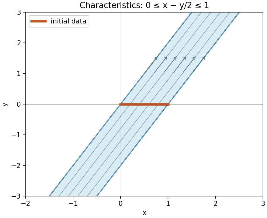
The data segment determines the solution throughout the strip swept out by its characteristics
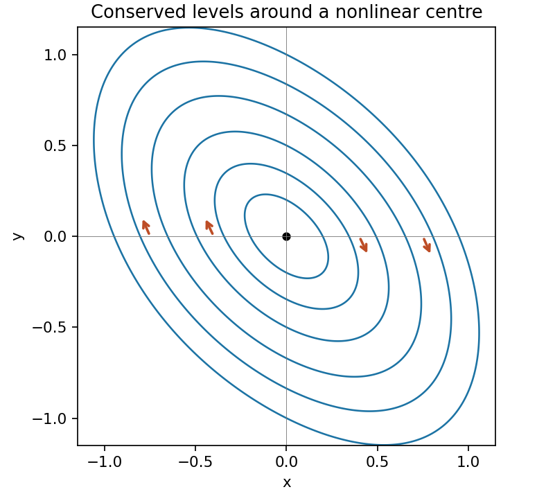
. Details. An equilibrium has from the first equation. Substitution in the second gives , so the origin is the only real equilibrium. Its Jacobian matrix isPurely imaginary linear eigenvalues alone do not classify the nonlinear equilibrium. Use insteadIts derivatives are and , so the vector field is . The chain rule gives . Therefore the nonstationary trajectories in the phase portrait lie on the level curvesThe quadratic part is positive definite, with eigenvalues and , so has a strict local minimum at zero. Small positive level sets are smooth closed ovals surrounding it, and the vector field never vanishes on them. They are periodic orbits. Thus the origin is a nonlinear centre, Lyapunov stable but not asymptotically stable. The near-origin ellipses have their long axis along . At with , the velocity points downward, fixing clockwise orientation.


Articles by others on the same topic
There are currently no matching articles.