Source: Mathematics Part A release, member
FOI-20210708-1 - Data/4301.pdf, dated 17 June 2013. All 35 source leaf parts are answered below.The department's solution-release policy excludes ordinary odd years; bounded exact-paper checks found no matching advertisement of full or selected worked answers. No parts are skipped.
The dual space is the vector space of all linear functionals on :Addition and scalar multiplication are defined pointwise. The annihilator of a vector subspace isIt is a vector subspace of : linear combinations of functionals vanishing on also vanish on .
Choose a basis of . Because , the list is linearly independent. Extend it to a basis of . A linear functional is specified uniquely by its values on a basis, so define to be zero on the and on every added basis vector other than , and set .
Then vanishes on every linear combination of the , so , whileThis proves that the annihilator of a vector subspace separates every vector outside the subspace from that subspace; no inner product or preferred coordinates are needed.
Every vanishes on , so . Conversely, suppose . Every is a linear combination , giving . If , part (b) supplies a functional in with , a contradiction. ThereforeFor the dimension statement, take a basis of and extend it to a basis of . Relative to the corresponding dual basis, a functional belongs to precisely when its first coefficients are zero. ThusIf , this says and the empty intersection is understood to be .
In the coordinate example choose the linear functionals and . Their kernels are the two coordinate planesTheir intersection is the stated axis, and .
The adjoint operator is characterized byThis identity works with either convention for which argument of the complex inner product is linear, provided the convention is used consistently.
For uniqueness, subtract the two given identities to get for every . Fix and choose . Then positive definiteness givesso . As was arbitrary, . The decisive fact is that a vector orthogonal to every vector, including itself, must be zero.
First suppose . For , choose with . For ,Thus . The direct sum of vector spaces gives , while the orthogonal complement has . Equal finite dimensions imply .
Conversely, suppose . Decompose arbitrary vectors as and , with and . Since is the indicated projection, and . Orthogonality makes the cross terms vanish, soTherefore satisfies the defining identity of its own adjoint operator. By uniqueness from part (a), . HenceThis is the characterization of an orthogonal projection among projections along a complementary subspace.
A Euclidean domain is an integral domain admitting a Euclidean function such that division with a smaller remainder is possible: for every and nonzero , there are withThus the Euclidean function measures progress in repeated division. Definitions which additionally normalize it to be nondecreasing under multiplication give the same class of Euclidean domains; the division property is the one needed below.
For the zero ideal, choose . Otherwise choose a nonzero for which the Euclidean function is minimal; the well-ordering principle guarantees such a choice. For any , perform Euclidean division:Because is an ideal, . A nonzero remainder would contradict the minimal choice of , so and . Thus . Conversely, implies , provingEvery ideal is therefore a principal ideal; in particular, a Euclidean domain is a principal ideal domain.
For the Gaussian integers, use the Gaussian normTo identify the ideal, note that is even if and only if have the same parity. AlsoThis quotient is a Gaussian integer precisely when have the same parity. Therefore the prescribed set consists exactly of the multiples of , givingAny associate of would generate the same principal ideal.
Under the assumed continuous real differentiability, the necessary and sufficient conditions are the Cauchy-Riemann equations at every point of :Necessity follows by computing the complex derivative along real and imaginary increments. For sufficiency, real differentiability gives the first-order expansionThe Cauchy-Riemann equations turn the linear part into , so the complex derivative exists and equals . Thus is a holomorphic function on .
At any , take sufficiently small so . The complex difference quotient isHence the complex derivative exists at every point of the punctured plane, andThe excluded point is essential to the domain statement: the reciprocal has a simple pole there.
Write . Both moduli are nonnegative, so squaring preserves their strict inequality:ThusThe boundary is the perpendicular bisector of and in the complex plane; the strict inequality selects the half-plane containing .
Use the reciprocal Möbius transformationIt is a holomorphic function on by part (b). For ,Part (c) now gives if and only if , so . Conversely, because . For any , put ; the same identity gives , so and . Finally, reciprocation is injective on nonzero complex numbers. This proves bijectivity, with inverseThe inverse is also holomorphic, so this is a biholomorphism.
For a piecewise continuously differentiable contour , the contour integral is defined byIf the contour has corners, integrate on its finitely many differentiable pieces and sum the results. The integral on the right is taken componentwise as an ordinary real-parameter integral of a complex-valued function. The factor encodes both the speed and orientation of the contour.
Choose the continuous argument with values in and defineIts branch cut is the nonpositive imaginary axis, including zero, exactly the removed ray. Locally away from that ray, the Cauchy-Riemann equations or the local inverse of the exponential show that it is a holomorphic logarithm, with derivative and . The chosen interval fixes the additive ambiguity by integer multiples of .
Use the branch from part (b) and close the real interval with the upper semicircle, oriented counterclockwise. For , the number has positive imaginary part, so the numerator is a holomorphic logarithm throughout a neighbourhood of the contour and its interior. The branch point lies strictly below the contour. The only enclosed pole ofis the simple pole at , with residueTo justify discarding the arc, take . On it, lies between and , and the argument has bounded absolute value. HenceThe real-axis integral is absolutely convergent, since its integrand is at infinity and has no real singularities. The residue theorem therefore givesFinally, . Taking twice the real part yieldsThe branch choice affects the first integral's imaginary part; the second integral is real and independent of that choice.
An isolated singularity at means that is holomorphic in some punctured disk , while itself is an excluded point or a point where the given function is not holomorphic. There are no other singularities arbitrarily close to . By Laurent's theorem, the function has a unique Laurent series on that punctured disk:The negative-power terms form its principal part of a Laurent series.
A removable singularity is an isolated singularity for which the function on the punctured disk extends to a holomorphic function on the full disk, by assigning or correcting its value at . In Laurent series terms,The remaining power series defines the extension with value at . Conversely, a holomorphic extension has a Taylor series there, so uniqueness of the Laurent series forces all negative coefficients to vanish.
A pole of order at has finitely many negative powers in its Laurent series, the lowest being exactly :Equivalently,Thus has a holomorphic extension with nonzero value at , whereas multiplying by any smaller power does not remove the singularity.
A zero of order at means that is holomorphic near andEquivalently its Taylor series starts with the nonzero coefficient of , soUnlike a pole, a zero is a regular point of the function itself; its reciprocal has a pole of the corresponding order.
By the finite-order zero factorizations,with holomorphic near . Shrinking the disk if necessary, continuity ensures never vanishes there, so is holomorphic and nonzero at . ConsequentlyIf , the exponent is , with a holomorphic nonvanishing factor. Hence
With the same factors, if , thenhas no negative power and extends holomorphically across . Thus its apparent singularity is a removable singularity, with extension valueFor the extended quotient has a zero of order ; for the extension is nonzero.
The complex sine has simple zeros exactly at , , because and . Hence the denominator has a zero of order three at each of these points and nowhere else.
At , the numerator has order two, so the quotient has a simple pole. Indeed its leading term is . At , the numerator has order one, so there is a pole of order two. At , the numerator has order three, cancelling the denominator's order-three zero, so the singularity is removable. Its extension value isAt every remaining , the numerator is nonzero, giving a pole of order three. Thus the complete finite-plane classification isAway from this discrete set the denominator is nonzero, so the quotient is holomorphic.
Collect the two dependent variables in a column vector. The vector field and initial vector areThe given system of ordinary differential equations is then with . Both components of are continuous on all of , since their denominators are at least one.
Each denominator is at least one and positive, so each component of lies in . Taking the maximum norm therefore givesThis is a global bound, so in particular the constant is valid throughout the specified cube.
For and ,Apply this to the first component with , , . The reverse triangle inequality givesFor the second component use , , to obtain . Taking the maximum yieldsThus is globally Lipschitz continuous in the dependent vector, uniformly in , with Lipschitz constant . Differentiability of the absolute-value function at zero is unnecessary.
A Lipschitz condition here is uniform in the independent variable: there is a finite constant such that, whenever both and belong to the cube,The same must work for every allowed . Part (c) proves this with . This controls changes in the dependent variables; no Lipschitz condition in is required for the Picard-Lindelöf theorem.
The quantitative Picard-Lindelöf theorem applies on a rectangle , . Suppose is continuous there, bounded in maximum norm by , and uniformly Lipschitz continuous in . Then the initial value problem , , has a unique solution onwith the usual interpretation if . The solution remains in the dependent-variable ball. Its endpoints are included when is continuous on the closed rectangle, as here. Equivalently, existence first on every smaller interval and the derivative bound give extension to those endpoints.
For the given cube, and . Thus the theorem gives once a bound and a uniform Lipschitz constant have been established. The theorem does not require : convergence of Picard iteration can be proved by factorial estimates or by using successive shorter intervals.
The vector field is continuous on the cube. Part (b) gives , and part (c) supplies a uniform Lipschitz constant . In the quantitative Picard-Lindelöf theorem, the independent-variable half-width and the dependent-variable radius are both one, soThereforeThe global derivative bound also makes the cube condition explicit. Along any solution segment starting at the initial point,Thus it cannot leave the dependent-variable ball before . Bounded derivatives give limiting endpoint values, and local existence extends to them because is defined continuously on all space. Uniform Lipschitz continuity ensures that all such local pieces agree on overlaps, proving uniqueness throughout the closed interval.
For , the discriminant is , so the equation is an elliptic partial differential equation, already in the canonical Laplace equation form .
For , the discriminant is , so it is a hyperbolic partial differential equation, the wave equation . Introduce characteristic coordinatesThen and , givingOn , the discriminant vanishes and the principal part has rank one; the degenerate parabolic type is . This is an interface line, rather than an open parabolic subdomain. ThusThis is a mixed-type partial differential equation. The classification concerns the principal part and remains meaningful even though the coefficient jumps at the interface.
In the lower triangular region, the characteristic coordinates obey . Integrating the canonical wave equation givesOn the right characteristic edge, and , so its prescribed value gives . On the left edge, and , giving . At the common vertex the two values agree and equal zero; hence .
Adding the two edge identities and subtracting this vertex identity determines the entire solution:The apparent freedom to add a constant to and subtract it from does not change . Every classical lower-region solution has the displayed separated form, so these two characteristic boundary traces determine it uniquely. Substitution into and into both edge values directly verifies existence.
The lower formula has a smooth continuation as a function of , and on it has trace . Its second tangential derivative iswhich vanishes at . Hence the continued lower formula satisfies the equation restricted to the interface, where the formal equation is .
Assuming the solution itself is continuous across the interface, the upper region therefore has the Dirichlet boundary value problemThe zero function satisfies these data. The maximum principle for harmonic functions, applied to both and , proves uniqueness among harmonic functions continuous on the closed rectangle. Thus is the continuous upper continuation. Satisfaction of the degenerate interface equation does not impose continuity of the normal derivative; that is the issue in part (d).
Differentiate the uniquely determined lower solution and the zero upper solution:Their one-sided traces areThey disagree, for example at , so the normal derivative is not continuous across the interface. The jump, defined as upper trace minus lower trace, is . It vanishes at the two interior points , but not identically on the interface.
This illustrates that continuous transmission need not preserve normal derivatives. In fact, at any point where these traces differ, the two-sided first derivative with respect to does not exist. The resulting function is continuous and smooth separately on each open side, but is not globally . Consequently a globally classical solution satisfying all these data cannot exist. The calculation in part (c) evaluates the smooth lower formula on the interface; it does not supply the missing cross-interface regularity.
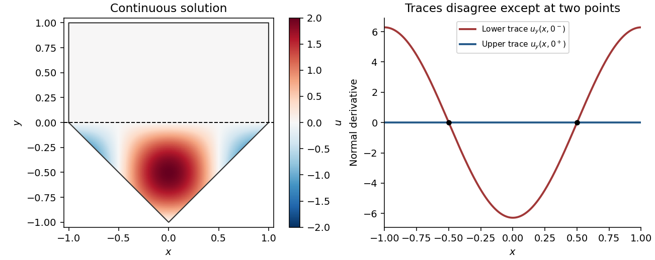
Continuous piecewise solution and unequal normal derivative traces
. Details. 
Inside the half-plane of convergence, the differentiation theorem for the Laplace transform permits differentiation with respect to the transform variable. Since ,Repeating the argument, or applying induction using , givesThe identities hold for , within the stated convergence half-plane. The usual transform differentiation theorem uses an interior margin in the real part of to control the polynomial factors in ; it makes no assertion on the boundary .
Integrating the complex exponential and taking its even and odd combinations gives the standard Laplace transformsFor example, for , and the real sine and cosine identities follow by combining the two signs of .
Apply part (a) once to the cosine transform and twice to the sine transform:All four transforms are valid on the stated right half-plane.
Write and . The zero initial data and the Laplace transform of a derivative give . Transforming the forcing with part (b),ThereforePart (b) with gives . Comparing coefficients and using uniqueness of the Laplace transform,As a direct check, , so both initial values vanish. Differentiating once more cancels the terms in , leaving as required. This also checks the factor in the inverse transform.
This paper was printed as Algebra, Analysis and Differential Equations I and was shared by mathematics and mathematics and statistics. Source: released examination archive, member
FOI-20210708-1 - Data/4301 (1).pdf, pages 1–4. The examination took place on 18 June 2012. No mark allocations are printed. The solutions cover all nine questions.The dual space consists of the linear functionals on the original vector space, with addition and scalar multiplication defined pointwise:The dual map acts by function composition with :For , its value is . The composite is a linear functional because both and are linear maps. Moreover , so the dual map is itself a linear map. Its direction is reversed because a measurement on the output of becomes a measurement on its input.
The annihilator of a vector subspace consists of the linear functionals that vanish on every element of that vector subspace:For the dimension identity, choose a basis of and use basis extension to obtain for . A linear functional is determined by its values on these basis vectors. Belonging to the annihilator of a vector subspace sets its first values to zero and leaves its last values arbitrary. Equivalently the last elements of the dual basis form a basis of .
For a linear functional , the definition of the dual map givesThus the kernel of a linear map is precisely the annihilator of a vector subspaceWrite , and . The rank-nullity theorem, the dimension formula for an annihilator of a vector subspace, and giveApplying the same dimension formula in givesFinally, if and , then . Therefore . These are finite-dimensional vector subspaces of equal dimension, so inclusion is equality:This is the dual image and kernel annihilator identity.
A diagonalizable matrix over the field admits an invertible matrix with entries in such thatEquivalently, the vector space has a basis of eigenvectors of . Indeed, says that each column of is an eigenvector with the corresponding diagonal entry as its eigenvalue. Requiring the basis and eigenvalues to lie in makes the choice of field essential.
Expansion down the last column gives the characteristic polynomialThe quadratic polynomial has roots , which are not rational numbers. For example, the rational root theorem restricts any rational root of this monic integer polynomial to or , and neither works. If had a diagonalization over , its characteristic polynomial would be a product of linear factors with rational numbers as their roots. It is not, so is not diagonalizable over .
Articles were limited to the first 100 out of 451 total.
Articles by others on the same topic
There are currently no matching articles.