Past exam of the approximation theory and finite element methods course of the University of Oxford / 2008 (C12.2, DMAC 2489, DMSU 2489)

Put $x=\cos \theta$. The trigonometric identitygives the Chebyshev polynomial recurrence $T_{n+1}=2x{T}_n-T_{n-1}$. Starting from $T_0=1$ and $T_1=x$, successive substitution yieldsThe recurrence also proves by induction that $T_n$ is a polynomial of degree $n$, with leading coefficient $2^{n-1}$ for $n\ge 1$.

For $n\ge 1$, set $p=2^{1-n}{T}_n$. It is monic by part (a), and its supremum norm on $[-1,1]$ is $E=2^{1-n}$. At the $n+1$ successive extreme points $x_j=\cos (j\pi /n)$ it alternates between $E$ and $-E$.

Suppose a monic degree-$n$ polynomial $q$ had $\Vert q{\Vert }_{\infty }<E$. At each $x_j$, the difference $p-q$ would have the sign of $p$. These signs alternate, so the intermediate value theorem forces a root in each of the $n$ successive gaps. But the leading monic terms cancel, making $\mathrm{deg}(p-q)\le n-1$, a contradiction. ThereforeThis is the monic monic Chebyshev extremal polynomial. The positive-degree restriction matters: at $n=0$ the printed scaling gives the constant two, while the only monic constant is one, so that version is false. The customary theorem uses $n\ge 1$.

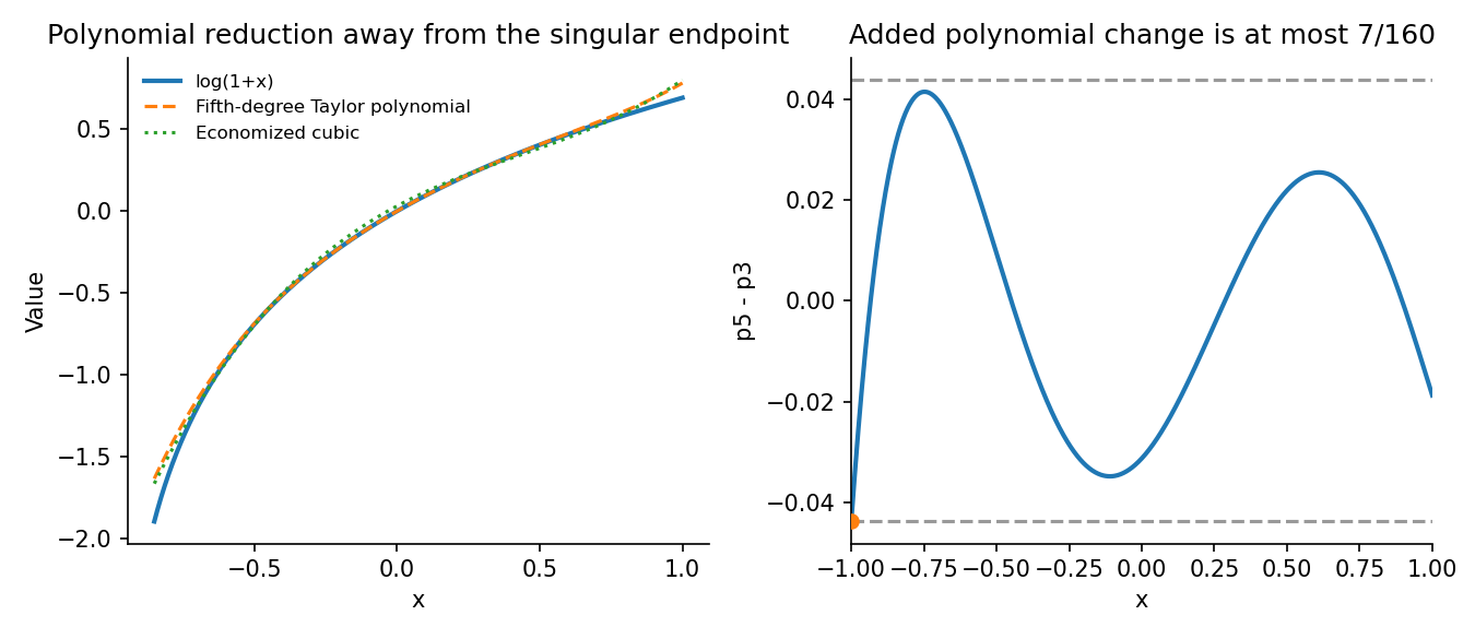
Expand the fifth-degree Taylor polynomial $p_5$ in Chebyshev polynomials, using the identities for powers obtained from part (a):Delete the last two Chebyshev terms and convert back to powers. The economized cubic isSince $|T_j|\le 1$,Equality holds at $x=-1$, where both deleted terms have negative sign. Thus the economization changes the polynomial by at most $7/160$, exactly in supremum norm on $[-1,1]$.

For the target itself, $|\log (1+x)-p_3(x)|\le |\log (1+x)-p_5(x)|+7/160$ wherever $x>-1$. The logarithm is singular at $-1$, so its total uniform error on all of $(-1,1]$ is infinite; the finite estimate concerns the additional polynomial change, or the increase on any smaller interval where the original error is bounded.

Use the standard convention that the orthogonal polynomials are nonzero. Their exact degrees then follow from the stated assumptions by induction: ${\varphi }_0$ is a nonzero constant, and if ${\varphi }_0,\dots ,{\varphi }_{r-1}$ span $P_{r-1}$, a nonzero ${\varphi }_r\in P_r$ orthogonal to all of them cannot lie in $P_{r-1}$.

Let $t_1,\dots ,t_m$ be the distinct sign-changing roots of ${\varphi }_r$ in $(0,1)$, and put $q(x)={\prod }_{j=1}^m(x-t_j)$. Then ${\varphi }_{r}q$ has constant sign between and across all its roots, and is not identically zero. Because $w>0$ in the interior, ${\int }_0^{1}w{\varphi }_{r}q$ is nonzero. If $m<r$, orthogonality to $P_{r-1}$ would make this integral zero. Thus $m\ge r$.

A degree-$r$ polynomial cannot have more than $r$ roots counted with multiplicity, so all $r$ roots are real, simple, and strictly inside $(0,1)$. This is the standard zeros of orthogonal polynomials argument, with the positive weight ensuring strict noncancellation.

The displayed recurrence requires monic normalization, which is not explicitly stated in the preamble. Arbitrary independent rescaling of orthogonal polynomials preserves orthogonality but changes the recurrence coefficients. Choose their monic representatives for this and the following calculations.

Expand $x{\varphi }_n$ in the orthogonal polynomial basis:The leading coefficient of ${\varphi }_{n+1}$ is one. For $j\le n-2$, $(x{\varphi }_n,{\varphi }_j)=({\varphi }_n,x{\varphi }_j)=0$, because the second factor has degree below $n$. Thus only $j=n,n-1$ remain. Inner products giveThe last equality uses $x{\varphi }_{n-1}-{\varphi }_n\in P_{n-1}$. Rearranging yields exactly the three-term recurrence for monic orthogonal polynomials

For weight $x^2$, the moments are ${\int }_0^1{x}^{j+2}dx=1/(j+3)$. Monic orthogonalization gives ${\varphi }_0=1$ and ${\varphi }_1=x-(1/4)/(1/3)=x-3/4$.

For ${\varphi }_2=x^2+ax+b$, orthogonality to $1,x$ requiresSolving gives $a=-4/3$, $b=2/5$. HenceThese are the nodes for the two-node Gaussian quadrature with quadratic weight.

Exactness on constants and linear functions givesWith the nodes just computed, the solution isTo prove cubic exactness rather than merely moment matching, divide a polynomial $u$ of degree at most three by the monic ${\varphi }_2$:The weighted integral of $q_1{\varphi }_2$ vanishes by orthogonality, and its two nodal values vanish because the nodes are roots of ${\varphi }_2$. The remaining $r_1$ is integrated exactly by the two equations above. This proves Gaussian quadrature exactness through degree three.

For a real-valued linear error functional annihilating $P_n$, the Peano kernel iswhere $x$ is the argument on which the functional acts. Under the standard boundedness and extension hypotheses, the Peano kernel theorem statesFor example, a bounded functional on continuous functions, represented by a finite signed measure and extended to the truncated powers, has this representation. Quadrature error functionals have precisely this structure.

The source's bare linearity assumption on $C^{n+1}$ is not by itself a complete theorem hypothesis. Truncated powers need not belong to that domain, and interchange of the functional with an integral needs justification. For instance $X[u]=u^{(n+1)}(t_0)$ annihilates $P_n$ but would require a Dirac point mass rather than an ordinary integrable kernel. The statement above supplies the usual functional class needed for the requested theorem and applies directly to part (c).

If $K$ has one sign, the weighted mean-value theorem applied to the continuous derivative $u^{(n+1)}$ givesfor some $\eta \in [0,1]$. One may prove this by bounding the weighted integral between the minimum and maximum derivative values times the total weight, then using the intermediate value theorem. If the total weight is zero, the fixed-sign kernel is zero almost everywhere and the conclusion is immediate.

Apply the Peano kernel theorem to $u(x)=x^{n+1}$ to get $X[x^{n+1}]=(n+1)!{\int }_0^{1}K$. Consequently

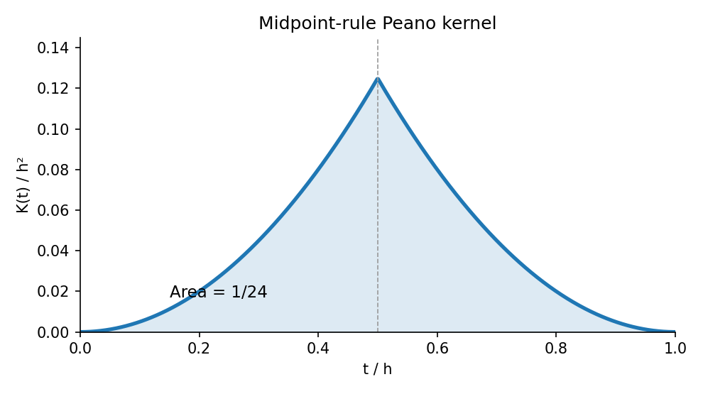
The midpoint error annihilates affine functions, so here $n=1$. Apply the functional to $(x-t{)}_{+}$:ThusIt is nonnegative, and symmetry gives ${\int }_0^{h}K=2{\int }_0^{h/2}{t}^2/2dt=h^3/24$. ThereforeFor a quadratic with constant nonzero second derivative equality holds, so this midpoint quadrature rule error constant is sharp.

The equioscillation theorem says that a best degree-at-most-$n$ polynomial approximation to a continuous real function on $[a,b]$ has $n+2$ ordered extreme-error points with alternating signs and equal absolute error. Conversely such alternation proves optimality. If the error is zero, the target is already a polynomial of the required degree.

For the single-point exchange in polynomial minimax approximation, start with $n+2$ ordered reference points $t_j$ and solve the linear systemfor the $n+1$ polynomial coefficients and $E$. Locate a point of largest absolute error on the interval. If its magnitude is no larger than $|E|$ within the desired tolerance, alternation certifies the approximation.

Otherwise insert that point and delete one old reference point so that the ordered signs still alternate. If the new point lies between two reference points, delete the neighboring point with the same error sign. If it lies outside the reference range, either replace the adjacent same-sign endpoint or, for opposite sign, insert it and drop the far endpoint. Solve again and repeat. This is the one-point Remez algorithm; a global extreme-error search is required for its stopping certificate, rather than merely checking the old reference points.

A $C^2$ piecewise cubic supported on $[0,ph]$ has the truncated-power representation with indices $0,\dots ,p$. Vanishing for $x\ge ph$ imposesafter expanding its cubic exterior polynomial; powers of $h$ cancel. For $p\le 3$, the Vandermonde matrix columns are independent, forcing every coefficient to be zero. For $p=4$, coefficients proportional to $(1,-4,6,-4,1)$ satisfy these conditions because a fourth finite difference annihilates cubics.

Normalize to get the Cardinal cubic B-splineAt its five support knots its values are $0,1/6,2/3,1/6,0$, so their sum is one. Thus four intervals are necessary and sufficient.

For $h=1/2$, the five translates active in the interior of $[0,1]=[0,2h]$ are indexed $-3,-2,-1,0,1$. Write $s(x)={\sum }_{j=-3}^1{c}_j{N}_j^3(x)$. Nodal interpolation givesAt the left endpoint the first derivatives of the three active functions are $-1/(2h),0,1/(2h)$, and their second derivatives are $1/h^2,-2/h^2,1/h^2$. The two remaining equations areTogether these five equations form the requested system; insert $h=1/2$ if numerical coefficients are desired. The first, fourth and fifth determine the first three coefficients, and the other two then determine $c_0,c_1$, so the system is nonsingular.

The source only assumes $u\in C[0,1]$, which need not have either endpoint derivative. The Hermite conditions require those derivatives to exist, or to be supplied as separate interpolation data. The nodal conditions alone remain meaningful for every continuous $u$.

The Sobolev space $H^1(0,1)$ consists of square-integrable functions whose weak first derivative is square-integrable, with norm $\Vert v{\Vert }_{H^1}^2={\int }_0^1(v^2+v^{\prime 2})$. Its one-dimensional representatives have well-defined endpoint traces.

Multiplying by $v\in H^1$ and integrating by parts givesThe two Robin conditions give $u^{\prime }(0)=u(0)$ and $u^{\prime }(1)=-u(1)$, so defineA weak solution is $u\in H^1(0,1)$ satisfying $a(u,v)=\ell (v)$ for every $v\in H^1(0,1)$. The boundary conditions are natural; no endpoint derivative is imposed in the trial space.

Since $\cos x\ge \cos 1>0$ on this interval,This proves coercivity on the full space. Trace continuity and Cauchy-Schwarz give continuity of the form, so the Lax-Milgram theorem also ensures a unique weak solution.

Let $V_h$ be the space spanned by all $N+1$ hats, including the endpoint hats. The solution in a conforming finite element space satisfies $a(u_h,v_h)=\ell (v_h)$ for all $v_h\in V_h$. The continuous form remains coercive and continuous on this subspace, so the discrete solution is unique.

With $u_h={\sum }_j{U}_j{\phi }_j$, its equations areThe formula is symmetric in $i,j$. For a nonzero vector $V$, the corresponding spline $v_h={\sum }_j{V}_j{\phi }_j$ is nonzero by basis independence, andThus $A$ is symmetric positive definite, proving algebraic solvability as well.

Testing against compactly supported smooth functions gives the distributional identity $u^{\prime \prime }=\cos xu-f$. The right side belongs to $L^2$, since $u\in H^1$ and $\cos x$ is bounded. Therefore $u^{\prime }\in H^1$ and $u\in H^2(0,1)$. This also makes the endpoint derivative traces meaningful, and integrating the weak form by parts recovers the Robin conditions.

The standard piecewise linear finite element interpolation estimate iswith constants independent of $h$. Hence $\Vert u-I_{h}u{\Vert }_{H^1}\le Ch\Vert u^{\prime \prime }{\Vert }_{L^2}$ for $h\le 1$. By Céa's lemma, with the fixed continuity and coercivity constants of $a$,The constant depends on the continuous problem but not on mesh refinement.

For any $v\in H^1(\Omega )$, expand $J(u+ϵv)$ in $ϵ$. Its linear term must vanish at a minimizer, givingThus the required functionals areThe form is continuous, symmetric, and coercive, with $a(v,v)=\Vert v{\Vert }_{H^1}^2$. Conversely, this weak equation implies $J(u+w)=J(u)+\frac{1}{2}a(w,w)$, so its unique solution is indeed the global minimizer.

For smooth $u$, Green's first identity rewrites the weak equation asCompactly supported test functions yield $-\Delta u+u=f$. Since the test space is the full $H^1(\Omega )$ and has unrestricted boundary trace, the remaining identity gives the homogeneous Neumann condition.

For a merely weak solution on a polygon, the normal derivative is understood as its weak flux trace. Here $\nabla u\in L^2$ and $\mathrm{div}\nabla u=u-f\in L^2$, so this trace is defined through Green's formula. It vanishes by the same identity. Thus the natural boundary condition is ${\partial }_{n}u=0$, without assuming global $H^2$ regularity on an arbitrary polygon.

Take $V_h$ to be all continuous functions affine on each triangle of the stated negative-diagonal mesh. No boundary value is fixed, because the Neumann condition is natural. The discrete problem isIts matrix is symmetric positive definite: the reaction contribution $\int u_h{v}_h$ removes the constant null mode that would occur for pure Neumann Poisson equations. Thus the solution exists uniquely.

For every $v_h\in V_h$, expand the quadratic functional about $u_h$ and use the discrete weak equation to remove its linear term:The continuous solution minimizes $J$ over the larger space $H^1$, so

Put $e=u-u_h$ and $V=\{v\in H^1(0,1):v(1)=0\}$. The primal solution and its finite element approximation lie in the same affine space with value one at the right endpoint, so $e\in V$. UseDefine the dual solution byEquivalently $z\in V$ satisfies $a(v,z)=(e,v)$ for every $v\in V$. Positivity of $p,q$ gives a unique solution, and one-dimensional regularity gives $z\in H^2$.

Then $\Vert e{\Vert }_{L^2}^2=a(e,z)$. The nodal interpolant $I_{h}z$ belongs to the homogeneous finite element test space, so Galerkin orthogonality gives $a(e,I_{h}z)=0$. Set $w=z-I_{h}z$. Using the primal weak equation,Integrate the derivative term separately on each element. Since $w$ vanishes at every mesh node, all endpoint flux and flux-jump terms vanish. ThereforeThe absence of jump terms here follows specifically from one-dimensional nodal interpolation; it is not an assumption that the finite element flux itself is continuous.

Let $p_{\ast }=\min p>0$, $q_{\ast }=\min q>0$, $q^{\ast }=\max q$, and $P_1=\Vert p^{\prime }{\Vert }_{\infty }$. Testing the dual equation with $z$ givesConsequently $\Vert z{\Vert }_2\le \Vert e{\Vert }_2/q_{\ast }$ and $\Vert z^{\prime }{\Vert }_2\le \Vert e{\Vert }_2/\sqrt{p_{\ast }{q}_{\ast }}$. From $p{z}^{\prime \prime }=qz-e-p^{\prime }{z}^{\prime }$,On an element of length $h_i$, the interpolation error vanishes at both endpoints and its derivative has zero mean. Two Poincaré inequalities giveApply Cauchy-Schwarz to the residual identity, with factors $h_i^2$ and $h_i^{-2}$:If the error is nonzero, cancel its norm after the regularity estimate; if it is zero the conclusion is immediate. One explicit reliable constant isThis proves the requested dual residual bound entirely in terms of the coefficient functions.

Compute $C$ from part (b), solve the finite element equations, and calculate the element indicators ${\eta }_i^2=h_i^4\Vert R_h{\Vert }_{L^2(I_i)}^2$. Let $\eta =({\sum }_i{\eta }_i^2{)}^{1/2}$. Stop when $C\eta <\mathrm{TOL}$; the proved reliability bound then certifies the requested true-error tolerance.

Otherwise mark elements carrying a chosen fraction of the total indicator, bisect them, and repeat. To ensure termination as well as a valid stopping test, include a uniform-refinement safeguard, for example bisect every element on every second unsuccessful pass. This preserves adaptive refinement on the other passes while forcing $h_{\max }\to 0$.

Here termination can be justified directly. On each element $R_h=f+p^{\prime }{u}_h^{\prime }-q{u}_h$, so its global $L^2$ norm stays bounded if $\Vert u_h{\Vert }_{H^1}$ stays bounded. That stability follows from coercivity after subtracting the fixed lift one at the right endpoint. HenceThe safeguarded algorithm therefore eventually satisfies the strict tolerance. Reliable numerical evaluation of the residual integrals, or an upper bound for their quadrature errors, is part of using the certificate in an implementation.

Use the full continuous piecewise linear space $V_h\subset H^1(0,1)$, including endpoint basis functions, because the boundary conditions are Neumann. DefineChoose $u_h^0$ as the $L^2$ projection of $u_0$ onto $V_h$. For each time step seek $u_h^{m+1}\in V_h$ withThis is the conforming Crank-Nicolson method. The reaction coefficient and the diffusion are both treated at the midpoint; integration by parts has removed the boundary flux through the homogeneous Neumann condition.

Test the discrete equation with $v_h=u_h^{m+1/2}$. The identity $(a-b,a+b)=\Vert a{\Vert }^2-\Vert b{\Vert }^2$ yieldsSince $e^x\ge 1$ on the interval, $a(v,v)\ge \Vert v{\Vert }_{H^1}^2$. Therefore the requested inequality holds:Discarding the nonnegative second term and iterating proves $\Vert u_h^m{\Vert }_2\le \Vert u_h^0{\Vert }_2$ for every positive $\Delta t$, with no restriction relating it to $h$. This is unconditional $L^2$ stability; the initial projection also satisfies $\Vert u_h^0{\Vert }_2\le \Vert u_0{\Vert }_2$.

Write $u_h^m={\sum }_i{U}_i^m{\phi }_i$ and define the mass matrix and reaction-diffusion stiffness matrixThen each step isBoth component matrices are symmetric, so $A$ is symmetric. For a nonzero coefficient vector $v$, its finite element function $v_h$ is nonzero andThus $A$ is also positive definite and every update has a unique solution. Because nonneighboring hats have disjoint interior supports, the matrix is tridiagonal in nodal order.