Solutions to all three questions of the University of Oxford Differential Equations II paper, sat on 22 June 2023. Source: released examination PDF, parent PDF pages 118–120; questions on pages 119–120. Question statements are omitted. In Question 2(b), the usual interpretation that the forcing extends continuously to the closed interval is distinguished from continuity only in the interior.
The characteristic equation of the linear ordinary differential equation is , with roots . A real pair of homogeneous solutions is thereforeTheir Wronskian, with the convention , isThus the two functions are linearly independent throughout the interval and span its homogeneous solutions.
Use the unweighted inner product . Two applications of integration by parts giveThe given boundary conditions set at both ends, but leave and independently variable. The remaining boundary term vanishes for every admissible precisely when . Consequently the formal adjoint and the boundary conditions specifying the adjoint operator are
Set . To construct the Green's function from a Dirac delta function, require and zero endpoint values. Away from , the homogeneous solutions satisfying the left and right boundary conditions are respectivelyWrite for and for . A discontinuity in would generate a derivative of the Dirac delta function, which is absent from the desired equation. Thus is continuous. Integrating that equation through then gives the jump conditionThe resulting two equations are and . Since the Wronskian , they giveBoth endpoint values vanish. At , subtracting the two first derivatives gives , verifying the sign and normalization of the Dirac delta function.
The homogeneous solution already has the prescribed endpoint values. Thus has zero boundary conditions and satisfies . The Green's function givesEquivalently, splitting the integral at gives the explicit formulaAny difference between two solutions would be with zero endpoint values, forcing . The displayed solution is therefore unique.
At , the nonzero homogeneous solution satisfies both zero boundary conditions. Thus the boundary value problem has a nontrivial kernel and cannot have an inverse for arbitrary forcing.
More directly, the adjoint operator has the zero-endpoint homogeneous solution . If an ordinary Green's function existed, the integration by parts identity would implyBut for . This contradiction rules out the Green's function for the unmodified operator. It is the Fredholm alternative obstruction.
The nonzero endpoint data contribute to the Fredholm alternative condition. With , the same integration by parts identity givesFor the specified forcing the left side is . HenceTo verify sufficiency, set . Direct differentiation gives . At this value of , a particular solution of is . The complete family obeying the two boundary conditions isThe arbitrary constant records the one-dimensional kernel; existence does not imply uniqueness here.
Put . After division by , the Legendre differential equation has coefficientsBoth are analytic functions at zero, so . At either , has a genuine simple pole; hence these are singular points even when makes vanish. However,and both products extend analytically across . By the regular singular point criterion for a second-order equation,None of the three specified points is an irregular singular point.
Use . The Legendre differential equation becomesSubstituting a Frobenius series , , gives the indicial equation : the indicial root zero is repeated. For , the coefficient of yieldsorFor the multiplying factor is nonzero. At it vanishes, so and all later coefficients are zero. Thus one solution is a polynomial of exact polynomial degree , including a nonzero constant when . Denote a chosen normalization by .
The linear recurrence relation determines every analytic coefficient from , so there cannot be a second independent analytic solution at . To see the required logarithm explicitly, reduction of order gives the second solution locally asNear , the integrand is plus an analytic function. After rescaling the second solution, its form is thereforeThe analytic remainder converges locally; its constant term may be set to zero by adding a multiple of . The nonzero logarithmic coefficient makes linearly independent of . This Frobenius expansion of the Legendre equation at an endpoint gives a Logarithmic Frobenius solution; the same endpoint calculation at explains why the independent Legendre function of the second kind is excluded when boundedness at both ends is required.
Write the operator in divergence form:The Legendre differential equation therefore givesThese are the eigenvalues of . With the common positive-sign convention for a Sturm-Liouville problem, use instead:This is a singular Sturm-Liouville problem, because vanishes at the endpoints. Bounded eigenfunctions select the nonlogarithmic branches and satisfy there. The Lagrange identity for a Sturm-Liouville operator givesThe eigenvalues are distinct, proving the orthogonality conditionThe weight is one. No choice of normalization of the Legendre polynomials is needed for this conclusion.
First take the usual endpoint-regular interpretation . Integrating the divergence form shows that has finite endpoint limits. A nonzero limit would make proportional to near that endpoint, forcing a logarithmically unbounded . Thus boundedness requires , and consequentlyThis is orthogonality to the constant eigenfunction , hence the Fredholm alternative condition. It is also sufficient under the stated endpoint regularity: putIf , the zero-mean condition gives . Hence the last integrand is bounded, so extends continuously to both endpoints. Any two bounded solutions differ by a constant: their difference solves , whose other solution is .
For the requested eigenfunction expansion, setThe Legendre polynomials span all polynomials, so their completeness follows from the Weierstrass approximation theorem. Projecting onto each eigenfunction gives for . The zero mode is free, while . Thus the full family isThe formula is unchanged by rescaling any . For the usual normalization , the facts on and , together with the Cauchy-Schwarz inequality, bound each summand by a constant times . The series therefore converges absolutely and uniformly. Its identification with the preceding integral solution avoids unjustified termwise second differentiation.
There is a source ambiguity: continuity only on does not supply the endpoint control used above. Even for integrable forcing, zero mean alone is insufficient. For example, letThis is continuous in the interior, absolutely integrable, and has zero mean because . Yet every candidate with zero endpoint values of haswhose integral diverges logarithmically in at each endpoint. Thus no bounded solution exists. For a merely interior-continuous , the exact criterion is that some constant makesbounded as approaches both endpoints. The Bounded solvability for the Legendre operator criterion above covers the intended regular forcing and makes this endpoint limitation explicit.
When , the forcing has nonzero integral , violating the Fredholm alternative condition. There is no bounded solution. Directly, integration gives ; cancellation of its logarithmic divergence at requires , while cancellation at requires .
For , the constant is a particular solution. Subtract it from any solution. The remainder satisfies the Legendre differential equation, whose general solution is a combination of and the logarithmically unbounded Legendre function of the second kind. Boundedness removes the latter coefficient, givingThe constant forcing is orthogonal to for , consistently with Orthogonality of Legendre polynomials and the Fredholm alternative.
Consider real roots. Every zero at is , , and its derivative is nonzero. For a regular perturbation, write . The Taylor seriesgives . Thus, through the requested order,There is no quadratic term. The exact parametrization also verifies completeness and the remainder order for .
Take . There are two real branches, on different scales. For a root tending to zero, the Taylor series givesThe dominant balance is , so a fractional-power root expansion yieldsMore precisely . An ordinary power series in integer powers of would miss this scale.
There is also a root escaping to positive infinity. Boundedness of the sine term makes the leading dominant balance . The nonzero branch isIndeed the equation rearranges to , which yields on this branch. The bounded oscillatory correction need not have a constant limiting value.
To check that these are all the real solutions, solve for the parameter:Positive values occur only on and ; are not roots. A useful exact derivative isIt vanishes only at isolated points, so is strictly decreasing on each of these intervals. Its endpoint limits are and zero on each interval. This monotone parametrization of sine perturbation roots gives exactly one root in each interval for every , proving that both asymptotic branches, and no others, have been included. If negative small parameters are allowed, the transformation reflects these two branches and gives all real solutions for that sign as well.
For the positive coefficient of , setting gives the reduced equation , with general solution . A fast decaying homogeneous solution of is , placing the boundary layer at the left endpoint. Thus use the right boundary condition for the outer solution: impliesThe dominant balance gives width . With the inner variable and , the exact rescaled equation isAt leading order, , so . The asymptotic matching condition sets , and sets . ThereforeThe additive composite expansion has zero overlap to subtract. Its graph starts at one, decreases steeply over , and then stays close to zero; its initial slope is . The right endpoint discrepancy is exponentially small. The left panel of the figure below sketches this profile. A right-end inner expansion would instead contain a growing term and could not repair the left endpoint mismatch.
With the negative coefficient of , the reduced equation is unchanged, but the fast mode now decays away from the right endpoint. Apply the left boundary condition to the outer solution, givingThe boundary layer still has width . Put and . The rescaled equation isIts leading inner expansion has . The asymptotic matching condition is , while . ThusSubtracting the overlap in the additive composite expansion givesIts graph starts exponentially close to one, follows the gently decreasing outer solution, and drops from near to zero in a right boundary layer of width . The right endpoint value is exactly zero; the left endpoint error is . Its right endpoint slope is , showing the rapid final descent.
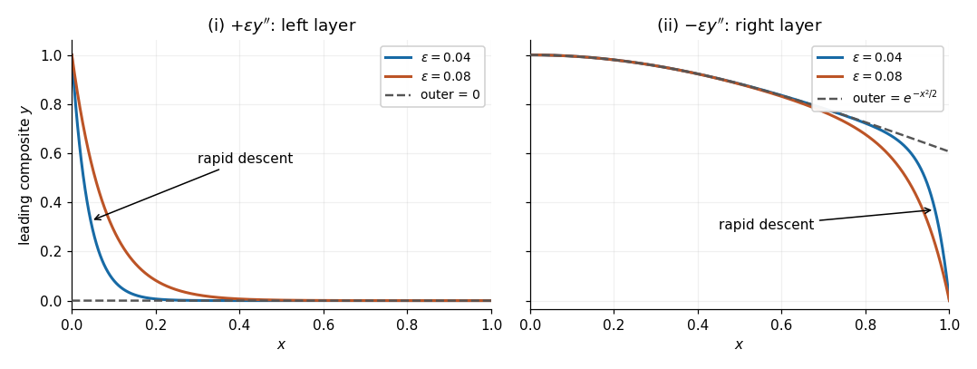
Leading composite profiles for the two signs of the highest derivative
. Original sketches from the derived additive composite expansions, for and . Left: the positive sign gives a left boundary layer and zero outer solution. Right: the negative sign gives a right boundary layer and the outer solution . Dashed curves show the corresponding outer solutions. Details.
Articles by others on the same topic
There are currently no matching articles.