Source: released examination bundle,
Part B 2007 11.pdf, pages 306–311. All six questions and both sections are covered. No mark allocations are printed.A pi-system is a collection of subsets closed under binary intersections: implies . Induction then gives closure under every nonempty finite intersection. A pi-system need not contain complements or unions.
The sigma-algebra generated by a collection is the smallest sigma-algebra containing that collection:The family being intersected is nonempty, since it contains the power set of . Intersections of sigma-algebras are sigma-algebras, so this definition has the asserted minimality.
The set function is countably additive if, whenever are pairwise disjoint and their union also belongs to ,The equality is in the extended nonnegative reals. To be a measure one also imposes and an appropriate domain such as a sigma-algebra.
The intersection of two nonempty members iswhich belongs to the collection. Any intersection involving the empty set is empty and is included too. Hence is a pi-system.
Conversely,The generated sigma-algebra contains both sets on the right and is closed under their difference, so it contains every open interval. By the given definition of the Borel sigma-algebra, the reverse inclusion follows. Therefore
Two sigma-algebras are independent if every event in one is independent of every event in the other:The same formula defines independence of the generating collections when restricted to their members.
Independence of the full sigma-algebras immediately gives independence of their generating pi-systems. For the converse, fix . On , define finite measuresThey have the same total mass and agree on by assumption. The supplied measure-uniqueness theorem makes them equal on . Thus the independence formula holds for every and every .
Now fix such an arbitrary . The measures and on have equal total mass and agree on . A second application gives equality on all of . This proves independence extended from generating pi-systems.
For each , the collection of events , together with the empty event, is a pi-system. Its generated sigma-algebra is , because the half-lines generate the Borel sigma-algebra and inverse images preserve intersections and the sigma-algebra operations.
The displayed probability identity says precisely that these two pi-systems are independent. Part (ii) makes and independent, which is the definition of independent random variables. Conversely independence of the random variables applies to the half-line events and gives the identity. Thus the joint cumulative distribution function factors exactly when the variables are independent.
Convergence in probability meansThe probability concerns each index separately; it does not require eventual closeness along almost every sample path.
For , convergence in Lp means the variables belong to andEquivalently the th absolute moment of the difference tends to zero. The analogous definition for uses the essential-supremum norm.
For events , the Borel-Cantelli first lemma states that implies . Indeed,These unions decrease to , so continuity from above proves the assertion.
The Borel-Cantelli second lemma states that independent events with satisfy . For every fixed , independence and giveContinuity from above shows there is probability zero of no event after . A countable union over gives probability zero of only finitely many occurrences. Independence is needed for this second conclusion, but not for the first.
For fixed and ,so there is convergence in probability to one. The absolute difference is exactly on the exceptional event, henceFor every this tends to infinity, so convergence in Lp fails. In contrast its first moment is , so convergence actually holds in .
There are exactly summands in , and the triangle inequality givesThe last step is convergence of arithmetic means of a sequence tending to zero. Thus in , and Markov's inequality gives
Let . These events are independent and . By the Borel-Cantelli second lemma, they occur infinitely often almost surely.
If had any finite sample-path limit, thenBut on , is either or , contradicting this convergence infinitely often. Therefore the averages have no finite almost sure limit. This is a rare-jump counterexample to a strong law with convergent first-moment averages.
A filtration is a nondecreasing family of sub-sigma-algebras: . It represents information available up to each time.
A martingale relative to the filtration is a sequence such that is -measurable, , andIterating conditional expectation gives the analogous identity between any two ordered times.
A stopping time is a random time taking values in the nonnegative integers together with infinity and satisfying for each . Whether stopping has occurred by time can therefore be decided from information available then.
The optional stopping theorem says that for a martingale and bounded stopping times ,For unbounded almost surely finite stopping times, additional hypotheses are essential. Sufficient versions include uniform integrability of the stopped martingale, or an integrable stopping time together with uniformly bounded increments. In the latter case, stop at and use and the dominated convergence theorem. This is bounded-increment optional stopping with integrable time.
Put . The hypothesis implies . Since and survival to implies survival to , the tower property of conditional expectation givesApply this at and use to obtainThis is a geometric tail bound from a uniform escape probability. The tail-sum formula for a nonnegative integer-valued variable now gives
Let be the first completion time of the word. A fresh gambler arrives before every throw with capital one, betting it all on the successive symbols . Each correct bet multiplies capital by six and each wrong bet loses it, so every bet is fair. A gambler who completes the word keeps the winnings.
At time , the gambler who bet on all four final throws has capital . The gambler who bet on the final two throws has correctly matched the suffix and has capital . There are no other survivors: the only nonempty suffixes of that are also prefixes are and . Thus the total surviving capital is .
To justify the expectation identity, independent blocks of four throws each have probability of equalling the pattern, so and . Total gambling capital minus the number of arriving unit stakes is a martingale with bounded increments before . Optional stopping therefore equates expected terminal capital with expected total stakes:This is the waiting time for a word in independent uniform symbols. The extra reflects the overlapping occurrence of the prefix at the word's end.
Write , and . In a one-step binomial options pricing model, absence of arbitrage requires . If , borrowing to buy the stock gives a nonnegative gain in either state and a positive gain in at least one. If , shorting the stock and investing the proceeds does the same. Conversely, strict inequalities give the risk-neutral probability , under which the discounted stock is a martingale; this excludes arbitrage at each node. Hence
Under a risk-neutral measure, the expected stock multiplier is the bank multiplier. With ,Thus , and the one-period effective return is also zero.
The terminal stock prices and European put option payoffs areLet be the risk-neutral up probability. Risk-neutral pricing and the supplied discounted-price condition giveso . Its roots are and ; only the first is a probability. ThereforeThe current put price is pounds. This interest rate is specific to part (c), and differs from the zero rate in part (b).
For matching European strike and expiry with no dividends, put-call parity gives . Using the rate and put price from part (c),As a check, only the call payoff is positive, at . Its risk-neutral expectation is , and discounting by gives the same value.
Return to and from part (b). An American put option is valued by the larger of immediate exercise and discounted continuation at each node. At time one with stock price , exercise gives zero, while continuation gives . With stock price , exercise gives , and continuation gives ; the holder is indifferent.
At time zero, exercise gives , while continuation gives . ConsequentlyIt is optimal to wait initially and at the up node; at the down node either exercise or waiting is optimal. At this zero interest rate, the European put also costs twenty pounds.
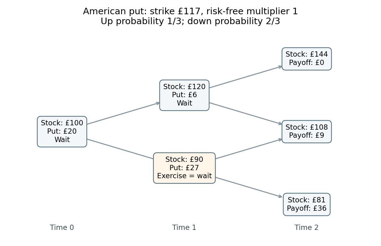
Backward induction for the American put when the risk-free multiplier is one and the up probability is one third. Each node shows the stock price and option value.
Details. 
Put . The linear combination starts at zero and has continuous paths. An increment over an interval of length is a linear combination of independent centred normal random variables, so is centred normal with varianceIncrements on disjoint intervals are independent, since they depend on disjoint increments of the two independent Brownian motions. These are the defining properties, so is a standard Brownian motion.
Cubing the supplied geometric Brownian motion solution gives . The moment-generating function of a normal distribution yields . Therefore
For this stock-dependent payoff, replace the stock drift by under a risk-neutral measure. Conditional lognormal moments then give, with ,This is the Power payoff in the Black-Scholes model. The delta hedge is shares, so the stock holding is worth . The rest is a bank position worth , or units of the bank asset. This gives a replicating portfolio; its self-financing identity follows from Itô's formula and the Black-Scholes pricing equation, and its terminal value is .
The full two-Brownian filtration contains an additional orthogonal noise direction, but this particular payoff is replicated using the traded stock and bank asset, so that extra noise does not affect its price.
Apply Itô's formula to , where . Since , the drift and diffusion areThusUnder the risk-neutral measure its drift becomes , as required for a traded, non-dividend-paying replicating asset.
For a call option on a power payoff, the replicating asset from part (c) has , volatility , and risk-neutral drift . The new payoff is therefore a European call option on , with strike . Applying the given Black-Scholes formula givesHere . Equivalently . It is the price process , rather than the raw power , that serves as the self-financing underlying for this application.
Under the physical probability, the stock has mean . Nonnegativity permits interchanging expectation and integration in the accumulated dividends. HenceTherefore
Let the accumulated bank account from past dividends beHolding one stock share and banking its dividends is a self-financing portfolio with wealth and . Doubling that strategy replicates the specified terminal payoff. Its price is thereforeIn particular its initial price is one hundred pounds. This illustrates banking stock dividends versus reinvesting them. The accrued-dividend term is known at time and belongs to the payoff defined from time zero; it cannot be discarded when .
For an ex-dividend stock, holding shares earns both and the dividend gain . Freeze locally in a self-financing hedge that is long the claim and short these shares. Itô's formula cancels its Brownian exposure, leaving drift . Its value is , so absence of arbitrage requires this drift to equal . Rearrangement gives the Black-Scholes equation with continuous stock dividends:With the given parameters,The physical drift cancels because the hedge removes the stock-price risk; the dividend payment remains in the stock's total gain.
The diffusion associated with the displayed pricing equation is . For , Itô's formula givesThe drift vanishes by the PDE. Under the usual integrability conditions for the payoff and solution, localization and conditional expectation make a true martingale; for polynomial-growth data the lognormal moment bounds provide the needed integrability. Applying the terminal condition yields the Feynman-Kac formulaThe printed diffusion contains an additional undefined factor multiplying . If literally retained, its second-order generator coefficient would be , so the requested representation would correspond to that different PDE unless . The formula above uses the volatility specified by the stock model and by part (c).
Under the pricing measure, the ex-dividend stock drift is . ThusA direct replication holds shares and reinvests every dividend into more shares. The share count grows at rate , reaching two shares at expiry, with no external cash input. This payoff contains only the terminal ex-dividend stock value, unlike part (b), which also includes the separately accumulated dividends.
Articles by others on the same topic
There are currently no matching articles.