Past exam of the mathematical physiology course of the University of Oxford / 2023 / 2

In the Hodgkin-Huxley model, $V$ is the intracellular-minus-extracellular membrane potential, $C_m$ is the membrane capacitance per unit area, and $I_{\mathrm{app}}$ is the applied inward electric current per unit area. A space clamp makes $V$ spatially uniform, leaving temporal ordinary differential equations. With outward ionic electric current positive, the capacitance balance is $C_m\dot{V}=I_{\mathrm{app}}-I_i$.

The variables $m,n,h$ lie between zero and one. They describe sodium activation, potassium activation and availability against sodium inactivation, respectively. Thus larger $h$ means less inactivation. Their voltage-dependent limiting values are $m_{\infty },n_{\infty },h_{\infty }$, and ${\tau }_m,{\tau }_n,{\tau }_h$ are their positive relaxation time constants.

Each ionic term has the Ohm's law form conductance times driving potential. The sodium term has instantaneous electrical conductance $g_{\mathrm{Na}}{m}^{3}h$, the potassium term has instantaneous electrical conductance $g_{\mathrm{K}}{n}^4$, and the leak term has constant electrical conductance $g_{\mathrm{L}}$. Here the $g$ constants are maximal electrical conductances per area, and $V_{\mathrm{Na}},V_{\mathrm{K}},V_{\mathrm{L}}$ are the corresponding reversal potentials. The factors $m^{3}h$ and $n^4$ arise from independent permissive gates in an ion channel. A conducting channel carries zero net ionic electric current at its reversal potential.

Use the three standard reduction assumptions: $m$ relaxes much faster than $V,n,h$ and can be replaced by $m_{\infty }(V)$; the two slower gates have the same time constant, ${\tau }_n(V)={\tau }_h(V)=\tau (V)$; and their limiting open fractions have a voltage-independent sum, $n_{\infty }(V)+h_{\infty }(V)=K$. The constant-sum assumption is essential: equality of two time constants by itself does not preserve a moving voltage-dependent sum.

For $q=n+h$, addition of the two gate ordinary differential equations givesThe specified initial condition is $q(0)=K$. Uniqueness for this first-order linear differential equation gives $q(t)=K$, hence $h=K-n$ for all time. The remaining two ordinary differential equations areThese assumptions give a planar reduction of the Hodgkin-Huxley model. The FitzHugh-Nagumo model keeps its fast activation and slow recovery variable geometry, approximating the voltage response by a cubic polynomial and the recovery response by a linear function after nondimensionalization. The polynomial equations in part (c) are a further model simplification; they are not an exact algebraic consequence of arbitrary original gate functions.

Assume $\epsilon >0$. At an equilibrium, $w=\gamma v=f(v)$, soThe nonzero roots areConsequently, with ${\gamma }_c=(1-a{)}^2/4$, there are three distinct equilibria for $0<\gamma <{\gamma }_c$, two distinct equilibria for $\gamma ={\gamma }_c$, and only the origin for $\gamma >{\gamma }_c$. At equality the two nonzero equilibria coincide; for $0<\gamma <{\gamma }_c$ they both have $a<v<1$. Geometrically, ${\gamma }_c$ is the maximum of the concave quadratic $(a-v)(v-1)$.

Since $f^{\prime }(0)=-a$, the Jacobian matrix at the origin isThus the origin is always asymptotically stable. Its eigenvalues areWriting ${\gamma }_N=(a-\epsilon {)}^2/(4\epsilon )$, the origin is a stable node for $0<\gamma <{\gamma }_N$ and a stable focus for $\gamma >{\gamma }_N$. At $\gamma ={\gamma }_N>0$ it is a degenerate node: the repeated negative eigenvalue has only one independent eigenvector, since the nonzero off-diagonal entry prevents $J_0$ being a scalar matrix. If $a=\epsilon$, then ${\gamma }_N=0$ and every permitted $\gamma >0$ gives a stable focus. This change from node to focus does not change stability and is not a Hopf bifurcation.

Take $\gamma >{\gamma }_c$ and let $\epsilon \to 0^{+}$ with the other parameters fixed. The nullclines are the cubic polynomial graph $w=f(v)$ and the line $w=\gamma v$. In the phase plane, $v$ increases below the cubic polynomial graph and decreases above it; $w$ increases below the line and decreases above it. The fast ordinary differential equation, in time $s=t/\epsilon$, freezes $w$ and gives $dv/ds=f(v)-w$.

At $w=0$, the fast roots are $0,a,1$. Their linear stability follows from $f^{\prime }(0)=-a<0$, $f^{\prime }(a)=a(1-a)>0$ and $f^{\prime }(1)=a-1<0$. Thus a fixed $0<v^{\ast }<a$ falls towards the resting branch, whereas a fixed $a<v^{\ast }<1$ rises towards $v=1$. If $v^{\ast }>1$, the first fast segment instead settles down towards $1$, followed by the same recovery excursion. The threshold $a$ is the leading singular perturbation threshold; finite-$\epsilon$ corrections matter for initial values approaching $a$ with $\epsilon$.

LetThese are the roots of $f^{\prime }(v)=0$. The outer branches $v<v_L$ and $v>v_R$ of the critical manifold are attracting under fast motion; the middle branch is repelling. The full excursion has four stages.

For this cubic polynomial, the landing point is explicit. Since $f(v)-f(v_R)=-(v-v_R{)}^2(v-v_J)$, comparison of the quadratic coefficients givesThus a graph of $v(t)$ has a rapid rise, a slowly falling elevated plateau, a rapid fall through zero to a negative undershoot, and a slow approach back to zero. The figure shows both the phase plane and a computed time trace. The smaller initial perturbation stays near the resting branch and produces no elevated plateau.

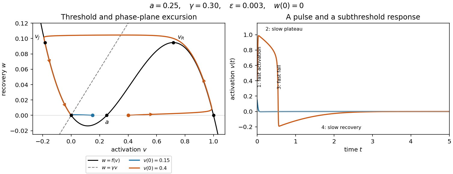
The four-stage description concerns the singular limit. Close to a simple fold point of a critical manifold, balancing the local quadratic activation term with the slow drift gives $\Delta v=O({\epsilon }^{1/3})$ and $\Delta t=O({\epsilon }^{2/3})$ for fixed parameters. These layers shrink compared with the slow phases and do not alter the leading time integrals below.

On an attracting branch of the critical manifold, $w=f(v)$ to leading order. The chain rule therefore givesThe initial fast segment ends at $v=1$, and the first slow phase ends at the right fold point of a critical manifold, $v_R$. HenceOn this interval $f^{\prime }(v)<0$ and $\gamma v-f(v)>0$. The integrand is negative, but the upper limit is smaller than the lower limit, so $T_1>0$. The numerator tends to zero at the fold while the denominator remains positive; the leading integral is finite. Fast segments and the fold delay give vanishing corrections as $\epsilon \to 0^{+}$.

The requested second phase is the second slow recovery phase, beginning after the downward fast jump. Its starting point is $v_3=v_J<0$, fixed by $f(v_J)=f(v_R)$, with the negative root chosen. Along it the same chain rule givesThe approach is to zero from below. Thus, if the printed cutoff $\beta$ is a signed value, it must satisfy $v_J<\beta <0$ and $v_4=\beta$. If $\beta$ denotes a small positive magnitude, the endpoint is instead $v_4=-\beta$. To express both conventions unambiguously, put $b=|\beta |>0$ and writeThere is no positive small endpoint on this leading slow branch. A positive cutoff would require a different event or finite-$\epsilon$ oscillatory recovery.

For bounded negative $v$ and $\gamma \gg 1$,Integration therefore gives the useful more detailed approximationTaking also $b\ll 1$, the leading logarithm isIndeed near zero, $f(v)=-av+O(v^2)$ and the slow equation is $\dot{v}=-(\gamma +a)v/a+O(v^2)$, so at fixed $\gamma$ the exact leading logarithmic coefficient is $a/(\gamma +a)$. Its large-$\gamma$ limit is $a/\gamma$, agreeing with the integral.

The order of approximation matters: first take the singular limit at fixed $\gamma$, then the large-$\gamma$ and small-cutoff limits. For simultaneous limits, a sufficient separation near rest is $\epsilon \gamma \ll a^2$. Otherwise the fast and recovery time scales merge, and these slow-branch formulas need not describe the late-time motion.