A density deficit in a flux tube is not by itself an instability calculation. For example, a straight magnetized tube in otherwise field-free gas at the same temperature has lateral balance . The perfect gas law then gives , so the tube rises unless some other force balances its weight deficit. This configuration simply lacks magnetostatic equilibrium. A magnetic buoyancy instability, in contrast, starts from a force-balanced atmosphere and asks whether a small allowed displacement grows. A balanced horizontal magnetic layer can be stable or unstable; the presence of magnetic pressure alone does not decide this.
Assume a smooth equilibrium, with downward gravitational acceleration , and write for the gas constant per unit mass. The ambient total pressure and force balance areWe use ideal magnetic flux freezing on the displacement time scale and rapid lateral pressure equilibration. A bodily displacement perpendicular to a straight horizontal tube does not change its length or bend its field. If its area is , conservation of magnetic flux and mass per unit length gives and . Thus the tube preservesEfficient heat exchange fixes its temperature to the ambient temperature at its new height, not to its original temperature. This is the thermal assumption that distinguishes the requested criterion from the adiabatic one.
Take a tube initially at and let . After a small upward displacement , let be the density it would have in lateral balance at . Its preserved and imposed local temperature giveAt the initial position . Differentiate this relation at :For the ambient atmosphere the same differentiation must also differentiate . It givesSubtracting isolates the actual displaced density contrast:The pressure-gradient force on the tube balances the weight of the displaced ambient gas, so its leading vertical buoyancy acceleration isThe coefficient multiplying is positive precisely when the tube becomes lighter on upward displacement. Thus the isothermal interchange criterion for magnetic buoyancy isWhere , this is simply , or . The squared form is independent of the field's choice of direction. Equality is neutral at this order, and the reversed inequality is restoring for these displacements. A layer with an interval satisfying the strict inequality admits local growing interchange disturbances under the assumed pressure/thermal equilibration. The calculation does not address field-bending undular modes, finite heat-transfer times or magnetic diffusion; those can change the criterion. In particular, the localized interchange criterion for a magnetized atmosphere with an adiabatic gas response is not interchangeable with this fast-thermal-exchange result.
Choose the poloidal magnetic field convention . The term regenerates this poloidal flux function from the toroidal magnetic field through the alpha effect. It represents a component of the mean-field electromotive force produced by correlated velocity and magnetic fluctuations. The shear stretches the poloidal vertical component into toroidal field, giving : this is the Omega effect. Both terms diffuse and damp the field. In a turbulent mean-field model, can denote an effective diffusivity including turbulent transport. The alpha-Omega dynamo approximation retains the shear-dominated toroidal source, and the kinematic dynamo assumption prescribes the velocity and coefficients without their Lorentz force feedback.
For a horizontal wavenumber and vertical wavenumber , set and seek amplitudes proportional to . The two modal equations areA nonzero mode requires the dispersion relationFor real nonzero , the root with positive real square-root part isThe other root has strictly negative real part. For there is no oscillatory feedback and both roots have real part ; the possible triangular-system prefactor cannot yield exponential growth.
Let and . The growing-branch exponent satisfiesConsequently the plane-layer alpha-Omega dynamo threshold at fixed isTo find its least value, differentiate :The unique positive solution is . The threshold diverges at both ends and , so this is its global minimum. HenceWith the usual positive- convention, the onset value is and exponentially growing waves exist for . Exactly at the threshold the real part is zero, so it is a neutral dynamo wave: the quoted minimum is the onset threshold, or infimum for strict growth, not a growing solution at equality. If signed is allowed, the growth condition concerns ; there is no smallest signed negative value among all growing cases.
The real field is obtained by taking the real part of a Fourier mode. Its phase is , so the horizontal phase speed is . Reversing the sign of reverses propagation, while leaving the growth threshold unchanged. Reversing gives the conjugate real-field representation.
Let be the magnitude of the downward gravity and write for the thermal expansion coefficient, to distinguish it from the dynamo coefficient of the previous question. The conductive state has , and . Its gravitational term is absorbed in a background hydrostatic pressure.
For the dimensional two-dimensional fields, choose the stream function and Cartesian magnetic flux function conventionsThese automatically give zero divergence. Define the Jacobian determinant bracket , so . The full magnetic flux function, including the imposed field, must be retained in the magnetic force; using the perturbation alone would lose its linear restoring term.
The scalar vorticity is . Also , and henceThe buoyancy perturbation is , whose curl in the direction is . Taking the curl of the momentum equation and multiplying by minus one eliminates pressure and therefore givesWe have restored in this dimensional expression. The printed magnetic force uses units in which , or equivalently a correspondingly rescaled field.
Use length scale , time scale , velocity scale , stream-function scale , magnetic flux-function scale , and temperature perturbation scale . Thus the dimensionless total flux function isHere now denote coordinates divided by , and the same notation in the second identity denotes the physical temperature. The dimensionless parameters for thermal-diffusion scaling of planar magnetoconvection areThese are the Rayleigh number, Chandrasekhar number, Prandtl number and magnetic-to-thermal diffusivity ratio. The nondimensional magnetic-force coefficient is , so omitting the factor would use a different magnetic parameter.
The resistive induction equation becomes . Since , its perturbation equation has source . Similarly, advection of the conductive temperature gradient gives , producing the source in the perturbation heat equation. The resulting nonlinear equations are thereforeThis derives both forcing signs from the background fields, rather than selecting them by a stream-function convention after the fact.
For the specified roll mode put and , the positive eigenvalue of minus the Laplacian on each spatial factor. Writeand take , , , with amplitudes depending on . These factors satisfy the printed boundary conditions: sine factors make the normal velocity and vanish at the required faces; the second derivatives of the velocity factors give the stress-free conditions; vanishes at the top and bottom and vanishes at the sides.
Discard quadratic perturbation terms. Since , the magnetic force linearizes to . The needed derivatives areThe heat and induction equations give and . In the vorticity equation, its left side is and its three right-side contributions are . Consequently, withthe three-amplitude vertical-field magnetoconvection system isPrimes now mean . They are genuine time derivatives, as the original PDF shows.
For its linear stability, seek amplitudes proportional to . Eliminating or taking the determinant giveswhereAssume the physical range , , . The Routh-Hurwitz stability criterion gives strict decay exactly when , and . At these hold. As increases, the first loss of stability can occur through a zero eigenvalue or a conjugate imaginary pair.
The stationary threshold isAt this value, withIf , the other two roots have negative real parts and the zero root is simple. Its derivative with respect to is . This is stationary onset; the reflection symmetry of the roll permits a generic pitchfork bifurcation. The linear calculation does not determine whether the nonlinear branch is supercritical or subcritical.
For oscillatory onset set , . Separating real and imaginary parts gives and . Solving the latter for yieldsA genuine Hopf bifurcation onset requires , soAt this threshold , giving the third root . The pair crosses transversely: differentiating at gives
The first instability of the conductive state is therefore stationary at if , or if and . It is oscillatory at if and . At , the two thresholds meet and : the frequency is zero and neither a simple pitchfork nor a nonzero-frequency Hopf test applies. The oscillatory marginality in vertical-field magnetoconvection formula must not be used where its frequency squared is negative.
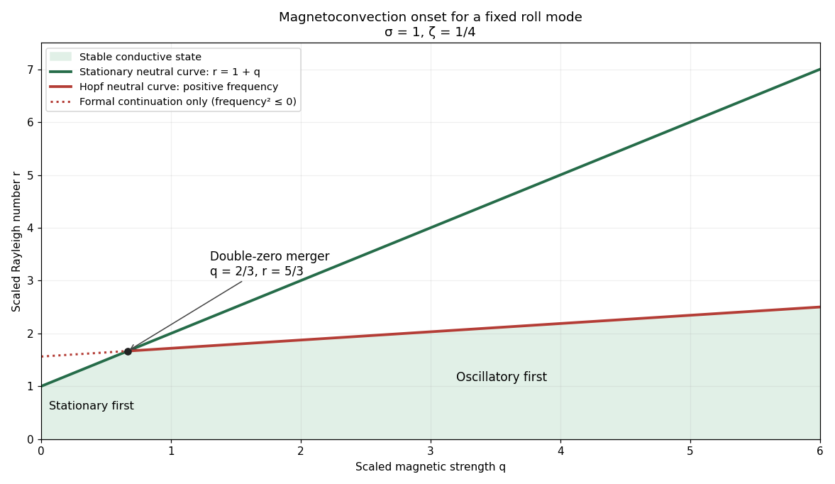
Stationary and oscillatory magnetoconvection neutral curves for Prandtl number one and magnetic-to-thermal diffusivity ratio one quarter, showing the double-zero merger and stable region
. Details. 
For conversion back to physical parameters, , while the dimensional Hopf frequency is . These are onset conditions for the specified spatial mode. Identifying the globally first mode would additionally require comparison over the allowed spatial modes. Nonlinear saturation and the stability of the bifurcating finite-amplitude states are not determined by this linear three-amplitude system alone.
Magnetic flux concentration and flux expulsion describe redistribution of an existing field, not necessarily creation of net flux. For a weak field in a prescribed conducting flow, the resistive induction equation isIts ideal part combines transport, stretching and compression:Thus a converging flow can intensify a component, and stretching can increase magnetic energy even if the signed net flux is zero. At large magnetic Reynolds number , diffusion is initially slow on the eddy scale, so magnetic flux freezing carries field lines with the flow. These statements do not imply that an ideal closed eddy can simply lose its initially enclosed flux.
The missing step is the production of small scales by differential circulation. In a two-dimensional incompressible eddy, the Cartesian magnetic flux function obeysDifferent streamlines have different circulation rates. An initially smooth field is wound into fine folds; diffusion and reconnection then smooth the variation of inside the eddy. As becomes nearly uniform there, its gradient and hence the interior magnetic field become small. The surviving flux lies mainly near the circulation boundary and adjacent separatrices, where stronger gradients remain. This is flux expulsion. With exactly zero diffusivity, field topology and the flux of material loops remain frozen, so a relaxed flux-free interior is not obtained by pure advection alone. Rigid rotation also fails to generate the differential winding responsible for this process.
The phase mixing in magnetic flux expulsion estimate makes the enhanced role of small diffusion explicit. If the angular-velocity gradient is of order , a wound radial wavenumber grows as . The accumulated damping exponent is of orderIt becomes order one atThis is much shorter than the large-scale diffusion time at large , but longer than one turnover time. It is a kinematic differential-shear estimate, not a universal time for every turbulent or rapidly evolving convection cell.
A related concentration mechanism occurs at converging flow boundaries. For a locally vertical bundle, conservation of flux gives , so reducing its cross-section increases . In a simple converging boundary region with strain rate , balancing strain and transverse diffusion givesThis is the thickness estimate for that local strain-diffusion model; it need not be the thickness or energy scaling of every closed-eddy flux-expulsion problem. Stronger field eventually exerts Lorentz force feedback and changes the flow. The equipartition magnetic field is a useful indication that the kinematic assumption can fail, not a universal upper bound on concentrated fields.
At the Sun's photosphere, hot upflows form solar granules, and their spreading horizontal motion transports weak vertical field toward cooler intergranular lanes and downflows. A thin-layer illustration, neglecting vertical transport terms, is . It gives : horizontal convergence intensifies the vertical flux density. This surface transport is related to the redistribution by convective eddies, but is not identical to the closed-streamline mechanism in the preceding planar example. Larger-scale supergranulation also gathers magnetic elements toward its boundaries, helping organize the solar magnetic network.
Concentration can be further intensified by compressible thermal dynamics. In the thin-tube picture of convective collapse, an unstable downward flow drains gas, reduces internal pressure and allows contraction at approximately conserved flux. Lateral balance then permits field stronger than the local kinetic equipartition estimate. This evacuation mechanism is excluded by a strict Boussinesq approximation. It is not a description of every evolving surface concentration: gas pressure, dynamic stresses and magnetic curvature can all matter when thin-tube equilibrium fails. The resulting strong, intermittent magnetic elements are associated with intergranular structure; their radiative appearance also depends on thermal structure and opacity. The organized fields of sunspots require a broader account of flux supply and magnetic feedback, rather than attribution to weak-field expulsion alone.
Thus convection redistributes and concentrates flux, finite diffusion enables classical expulsion, and nonlinear magnetic and thermal feedback determines the strong-field outcome. An expulsion argument alone neither supplies the original solar field nor establishes a self-sustaining solar dynamo.
Articles by others on the same topic
There are currently no matching articles.