Fluid-loaded plate. Use complex amplitudes with time dependence and take the velocity potential in the fluid above the elastic plate to be . Let and be the undisturbed mass density and speed of sound. The linearized Euler equations give ; the kinematic boundary condition is . We model loading from one fluid half-space, with no fluid loading on the other face. Loading by identical fluids on both faces instead doubles the fluid term below.
Define the Fourier transform and its inverse byThe Sommerfeld radiation condition selects , with and . Here and in the diffraction calculation below, the outgoing square root is specified by first taking . Draw a vertical cut upwards from and another downwards from , and putThus is analytic in the upper half-plane and in the lower half-plane. In the real-frequency limit,The Fourier transform contour follows the real axis with the limiting-absorption pole prescriptions. In particular, an outgoing propagating component has positive vertical wavenumber.
The kinematic boundary condition gives , so . Eliminating the fluid pressure from the bending balance gives the line-forced fluid-loaded bending plate kernelFor harmonic line force amplitude at the origin, the plate displacement and fluid velocity potential are thereforeAn arbitrary localized loading replaces by its Fourier transform. This representation both calculates the response and identifies its different wave components through poles and branch points.
For an observer , , with , the method of steepest descent uses the saddle point . At fixed angle away from grazing, the acoustic far field isThe spreading is that of cylindrical acoustic waves. The phase velocity parallel to the plate is : components with are supersonic in that sense and radiate, whereas those with are subsonic and exponentially decay normally to the plate. The latter have reactive fluid loading and zero mean normal acoustic energy flux.
There is also a real guided root . Indeed, , , andThe residue theorem then gives an outgoing displacement contribution . It transports energy along the plate while its fluid field decays as . Other zeros on continued sheets can describe leaky or resonant waves; branch point contributions describe near and grazing fields. A fixed-angle acoustic far field expansion is not uniform near the plate, where these components can matter.
For a propagating spectral component, write . Its upward normal velocity is and its pressure is . Applying Parseval's identity to the time-averaged acoustic energy flux gives the upward power per unit length of the forcing line:Equivalently, the integrand is with prefactor . Integrating the radial acoustic intensity of the far field over a semicircle gives the same expression. The input power also feeds guided waves along the plate, so it must not be identified with alone.
Rigid half-plane diffraction. Suppress the time factor and assume . Write , , and denote the incident spatial field by . The Helmholtz equation, Sommerfeld radiation condition, and square-root branches are as above. Across the open positive axis the scattered field and its normal derivative are continuous. Across the rigid negative axis its normal derivative is also continuous, while its potential can jump. Let be this jump, supported on . The transformed scattered field isThe jump transform is analytic in the upper half-plane. The absence of an even scattered component follows from derivative continuity and the outgoing condition. Its normal derivative on either face is .
On the negative axis this derivative must cancel . Since the Half-range Fourier transform of is , the Wiener-Hopf equation has the formwhere is the transform of an unknown function supported on and analytic in the lower half-plane. The incident pole lies below the Fourier contour. Divide by and perform pole subtraction in a Wiener-Hopf equation:The first term is upper analytic and the second lower analytic, since the latter's apparent pole cancels. Equality of the two continued sides gives an entire function. The finite-energy edge condition, with , and the decay of the transforms at infinity force that function to vanish by Liouville's theorem. ConsequentlyThis is the Wiener-Hopf solution of rigid half-plane diffraction with the present transform and time conventions.
Deforming to a steepest descent contour gives a residue from the incident pole precisely when . At that pole ; its residue producesThus the total geometrical optics field is plus a reflected wave in the upper reflection region; in the lower shadow region the scattered residue cancels , and outside that shadow the direct incident wave remains. This gives both the amplitude and the spatial support of the geometrical optics fields rather than merely naming a reflected wave.
For , , , the saddle contribution uses and . The diffracted wave isThe total field is to this order. This far-field expression applies away from the shadow/reflection boundaries . There the pole and saddle coalesce, and a uniform Fresnel integral approximation replaces the divergent separate terms by a smooth transition. The exact contour integral remains well defined.
Write the perturbation Stokes streamfunction as , with and nonzero . Its radial and axial velocity amplitudes are and . These automatically obey incompressibility. Linearizing the radial and axial Euler equations, with pressure amplitude , givesThusDifferentiating the first expression, the terms involving cancel. Equating the two expressions for proves the axisymmetric inviscid pipe stability equation:At the axis, finite smooth axisymmetric velocity requires , after choosing the irrelevant constant in the streamfunction. At the wall, impermeability gives . There is no tangential no-slip condition in this inviscid problem. A decoupled azimuthal disturbance satisfies and does not introduce a growing discrete mode when .
For real , suppose with , so division by is legitimate. Multiply the ordinary differential equation by , integrate, and apply integration by parts. The endpoint terms vanish by the preceding regularity and wall conditions, leavingTaking its imaginary part yieldsA growing temporal mode therefore requires a sign change of , rather than a sign change of alone. This is the cylindrical counterpart of Rayleigh's inflection-point theorem. If this derivative vanishes identically, the positive first integral rules out a nontrivial growing real-wavenumber mode as well. Isolated zeros without a sign change do not make the second integral vanish for a nonzero regular mode.
For the parabolic Poiseuille flow, is constant. Under the specified exclusion of critical levels, division givesSetting , or equivalently choosing in , turns this intoIt is the Modified Bessel differential equation of order one. Hence . Since tends to a nonzero constant at the axis, it gives a singular radial velocity and must be excluded. The admissible mode shape is thereforeFor , direct solution gives after axis regularity, and the wall condition again forces the trivial solution. For nonzero , the nonzero roots of are imaginary. Writing for the zeros of the ordinary Bessel function , the evanescent potential modes of inviscid Poiseuille flow areTheir perturbation vorticity vanishes: . These modes grow exponentially in one axial direction and decay in the other. They can describe end-forced or spatially localized potential fields, but neither sign gives a bounded normal mode on a whole infinite pipe. Moreover, the reduced radial equation contains no : it supplies no temporal eigenvalue condition. An arbitrary imaginary part assigned to here is consequently not evidence for a physical temporal instability.
The real-wavenumber calculation does exclude growing discrete axisymmetric modes of this inviscid profile. It does not establish every form of stability: singular neutral disturbances with in the range of , transient dynamics, non-axisymmetric disturbances, and finite-amplitude transition require separate treatment. The exclusion specifically removes the inviscid continuous spectrum.
With viscosity, linearize the Navier-Stokes equations instead and eliminate pressure to obtain a fourth-order cylindrical counterpart of the Orr-Sommerfeld equation. Impose both and , with appropriate regularity at the axis. The resulting eigenvalue problem involves the Reynolds number and determines complex frequencies, rather than leaving arbitrary. Viscosity supplies diffusion, no-slip boundary layers and critical-layer regularization, so the inviscid sign argument alone no longer decides its spectrum. That observation does not imply that viscous pipe flow must have a growing linear eigenmode; finite-amplitude pipe transition is a different question.
The real-wavenumber dispersion relation has the explicit branchIts frequencies are real. A real-axis Fourier transform propagator multiplies every component by , of modulus one, so a square-integrable localized disturbance has constant norm. For sufficiently smooth localized data with an integrable Fourier transform, its pointwise amplitude also has a time-independent upper bound. In particular, there is no exponential growth along a fixed or moving ray.
The Briggs-Bers criterion makes the same conclusion while enforcing causality. Start the temporal inversion line at and the spatial inversion contour on the real axis. The spatial roots can be followed explicitly:Choose the principal logarithm along this upper temporal half-plane. Since , the root lies above the real axis; the root lies below it. Successive roots remain separated by . As is lowered, approaches the real axis when is real. The spatial contour is then indented beneath that root, as required by continuation from positive . No lower root meets it: their separation stays nonzero.
Algebraically,for every finite complex , so there is no finite spatial pinch point. The logarithmic singularity at sends roots to ; it is on the real-frequency boundary, not a positive-growth pinch in the upper temporal half-plane. The continuum of neutral poles is the real curve in the plane. It is reached as a causal boundary value, rather than producing an upper-half-plane singularity.
The figure follows neighboring spatial roots while lowering horizontal temporal contours. It shows why merely finding roots in both spatial half-planes does not establish an instability: those roots never collide across the inversion contour.
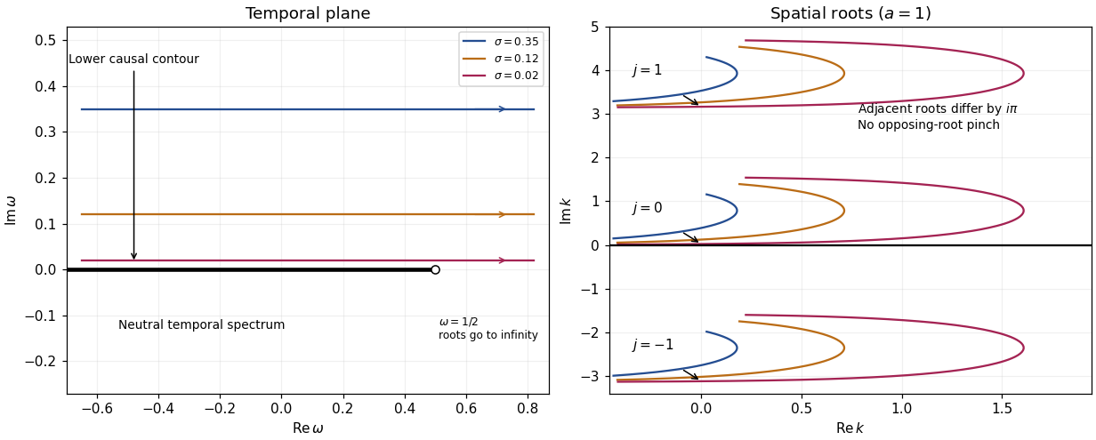
Causal temporal contours and nonpinching spatial roots of the triangular-jet dispersion relation
. Details. 
These modes have neither absolute wave-packet instability nor convective wave-packet instability; they are temporally neutral. Their positive real group velocity transports wave packets downstream. Nonreal spatial roots describe spatial continuation and evanescence, not temporal amplification. The exponential growth criteria concern the causal impulse response, not an unrestricted choice of a complex root.
Expanding the exponential for gives . Substitution of the plane wave in the model giveswhich is exactly the quadratic approximation to the dispersion relation.
For the slowly varying width, put and use the WKB approximationThe derivatives areAt leading order . On the downstream small-wavenumber branch writeso is independent of . The next order gives the slowly varying triangular-jet envelope transport equationIntegration therefore yieldsIndeed, . The requested power is the leading low-frequency envelope, not the exact finite-frequency exponent of the quadratic model. The corresponding leading field is this wave envelope times . Positive slowly varying width and separation from the zero of the local group velocity, , are needed for this WKB approximation. Extremely large can also invalidate replacing the exact exponent by .
Use mass conservation and conservative momentum conservation, with viscous stress defined so that its divergence is the viscous force:Differentiate the first equation in time and eliminate the momentum time derivative using the second. This givesSet and , where the reference values and are constant. Subtract to obtain the exact Lighthill acoustic analogyThe Lighthill stress tensor includes nonlinear momentum transport, departure from the reference linear pressure-density relation, and viscous stress. For an inviscid fluid the last term is absent. The derivation is an exact rearrangement of the conservation equations; treating the tensor as a known localized source is a subsequent approximation.
Convolution with the retarded acoustic Green function, followed by two integrations by parts in the source coordinate, yieldsFor the acoustic compact-source approximation, replace the distance and the source retarded time by and in the leading moment. Thus the integral is , where . In the acoustic far field, each spatial derivative acts predominantly on retarded time: , where . Derivatives of and of give lower powers of . The two retarded derivatives therefore giveThis is the compact acoustic quadrupole field, retaining its angular stress projection.
For the compact acoustic quadrupole Mach-number scaling, let the source length be , typical fluctuation speed be , and typical time be . The low-Mach number stress is , so and . ConsequentlyWith the geometric ratio separated, this is the stated fourth-power dependence. It assumes an advective source time scale and compactness . An externally driven source with an independent frequency does not acquire the same Mach power automatically.
Interpret the surface delta as , so integration against it gives a surface integral. If is signed distance, this equals the notation directly. This convention is needed because an arbitrary rescaling of the level-set function must not change the physical source.
Define the volume flux and total pressure force . Here is the rate of change of body volume, not the volume itself. The surface acoustic monopole contributes, in the acoustic compact-source approximation,The surface acoustic dipole contributesThe second term is a nonradiating near-field term and is smaller in the acoustic far field. Writing with the observation point fixed, the leading augmentation is thereforeThe printed dipole coefficient is missing a factor . The extra inverse speed follows from differentiating , and is required dimensionally: the printed expression with has the units of density times speed. This corrected acoustic loading noise term also agrees with the far-field acoustic force and stress moments. The monopole coefficient is unchanged.
Let and use for the source radius, reserving for observation distance. Incompressible spherical potential flow satisfies . Its velocity potential, tending to zero at infinity, and velocity areThe unsteady Bernoulli equation givesThe surface pressure is independent of angle. Hence the integrated surface force is zero, , and the leading compact surface dipole contribution vanishes. This also makes in the notation of the preceding part.
The volume flux is , so the acoustic thickness noise contribution isThe leading part is linear in the radial oscillation. Keeping the quadratic terms explicitly gives .
For the acoustic quadrupole, use . To leading quadratic order,ThusKeeping the instantaneous lower limit instead gives , whose leading small-oscillation term is the expression just obtained. Although the stress moment is isotropic, its contracted second derivative is not zero: .
For a sinusoidal radius perturbation , the leading compact radiation moments of a pulsating spherical bubble areWriting and , the quadrupole amplitude relative to the linear monopole is . The monopole also has a quadratic correction, ; the volume-stress quadrupole is smaller than this quadratic monopole correction by .
In the small-amplitude compact regime, the linear monopole dominates, the leading dipole is zero, and the volume quadrupole is weaker and begins at twice the oscillation frequency. The compact formulas require as well as a far observer. The stated small surface Mach number alone does not imply compactness. The incompressible near field has a decaying tail, but its stress moment is dominated by distances of order ; an acoustic matching region is still needed outside it. These are leading compact contributions, not a claim to retain every finite-wavelength correction at the smaller quadrupole order.
The positive drift places the boundary layer at the left endpoint. Set and impose the right boundary condition order by order. The leading ordinary differential equation is , so . At the next order,which integrates toThe outer limit at the left endpoint is two, so it cannot satisfy the left boundary value without a rapidly varying correction.
For the inner expansion use and . Its equations and boundary values areMatching the leading constant gives . The first-order forcing is then . A particular solution is , and matching determines the constant to be . Enforcing givesIn the overlap region the common expansion is . Adding the inner and outer approximations and subtracting that common part gives the uniform asymptotic approximationIt has error uniformly for , apart from an exponentially small endpoint adjustment of the same asymptotic irrelevance. At it equals one exactly, and at it differs from one only exponentially. The polynomial multiplying the exponential remains bounded on the inner scale.
There is an independent check from a first integral. The equation is , so its exact solution has the formwhere is selected by the right boundary value. Endpoint expansion of this integral gives , the same outer coefficients and the same inner expansion. This check also establishes the uniform order of the composite approximation without treating an inner residual as an outer estimate.
The negative drift moves the outflow boundary layer to . The first-order outer equation is . It must satisfy the left boundary condition, giving . This tends to two at the right endpoint.
Use . The leading inner equation is , and impose and on matching. Thus , and a leading uniform asymptotic approximation isFor higher accuracy, expand the drift as in the inner equation, solve the successive inhomogeneous equations, and match to outer corrections satisfying zero left endpoint data. There is no need for a left endpoint layer. Choosing the growing exponential at the wrong endpoint would prevent matching and is the reason the layer location matters.
Here the drift vanishes at the left endpoint. The outer equation is , giving after applying the right boundary value. The ordinary layer does not balance diffusion and drift: their balance selects instead.
For the square-root boundary layer at a vanishing drift, put . The inner equation isMatching requires a leading inner amplitude of order , so an inner expansion with an everywhere order-one leading term would be incorrect. This can be seen directly by integrating the original equation once:The right boundary value determinesIn the inner variable the exact representation becomesThe first term enforces , while the second is zero there and matches for large . One would expand this integral in the overlap region, determine successive outer terms from the right boundary, and subtract their common expansion. The endpoint layer has width and an interior peak, while its value at the endpoint remains one. This distinguishes it from the ordinary exponential layers in the two preceding cases.
Introduce the slow time and expand . At leading order writeThe first-order equation isIts resonant sine and cosine components must vanish by the solvability condition in the method of multiple scales. Let angle brackets denote a full-period average. The cosine projection of the nonlinear term is zero, since . The sine projection givesThis is the averaged oscillator damping by a power of velocity.
If is odd, defineThen , givingFor every fixed , these leading multiple-scale expansions are uniform on bounded slow-time intervals . The unforced phase remains to this order. A bounded first-order correction supplies the small adjustment to the initial derivative and initial displacement; it does not change this leading result.
If is even, the average of the odd power vanishes. Thus andThe first-order forcing has only a constant and even harmonics, so it produces no fundamental resonance. Its bounded particular solution can be supplemented by homogeneous sine and cosine terms to satisfy the initial conditions. There can be an frequency correction, but its phase accumulation is only on the present time scale. In contrast to the odd case, the even-power force is invariant under velocity reversal and the equation is reversible; calling it positive damping for both signs of velocity would be wrong. The mechanical energy identity makes the distinction clear:This is nonpositive for odd and changes sign for even ; its cycle average reproduces the amplitude equation above.
For large odd , the central binomial coefficient givesThis form reveals several time regimes. For , ; at , the amplitude change is only . For but , the leading change is . In particular, at it is only , despite the long elapsed time. High powers damp mainly near velocity maxima, and even a small amplitude reduction strongly suppresses subsequent damping.
An order-one amplitude reduction in the averaged law requires . Formally, gives , and for fixed odd its late envelope is an algebraic power . These exponential-in- time scales are predictions of extending the averaged law; the fixed-, bounded- multiple-scale error estimate alone does not establish uniform accuracy that far. A joint large-, small- approximation also needs control of the increasingly sharp nonlinear peaks, rather than assuming fixed- error constants are uniform. Taking fixed first and then examining the large- envelope avoids that unsupported interchange of limits.
Articles by others on the same topic
There are currently no matching articles.