Use natural units and the Minkowski metric . The Lorentz group isWrite a transformation near the identity as . The defining relation gives , so is antisymmetric. ChooseThere are independent real parameters: three spatial rotations and three Lorentz boosts. Differentiating with respect to shows it is constant and equals . Thus exponentiating these infinitesimal generators gives Lorentz transformations connected to the identity. The component they generate is the proper orthochronous Lorentz group , characterized by and .
The local exponential calculation alone establishes products of exponentials. The single-exponential assertion also holds here. Use the Lorentz spinor double cover , obtained by acting on as . Its determinant is the Minkowski norm. A lift with distinct eigenvalues is diagonalizable and has a traceless logarithm with eigenvalues , where . With repeated eigenvalues, choose between and so that the lift is with ; its traceless logarithm is . Since the two signs have the same Lorentz image, exponentiating the differential of the covering map proves every proper orthochronous Lorentz transformation is an exponential:It is not a global assertion about the disconnected improper components of .
For Dirac spinors, choose gamma matrices satisfying the Clifford algebra and setThe Clifford relations giveThey also give the stipulated Lorentz commutator with every replaced by : commute through the two gamma factors defining the other generator and collect the four terms. Consequently this is a representation of the Lie algebra of the Lorentz group, and exponentiation yieldsThe Dirac adjoint transforms as , since .
There is a global qualification: a spatial rotation through gives , while its Lorentz matrix is . Thus Dirac spinors form an ordinary representation of the double cover, and a double-valued representation of , rather than a single-valued linear representation of itself. Fermion bilinears are unaffected by this sign.
For a scalar field, and its derivative transforms as a covector. A Lagrangian density must have all Lorentz indices contracted into scalars using invariant tensors; arbitrary scalar potentials are allowed. For example the kinetic contraction and a potential are invariant. Lorentz invariance by itself does not restrict the potential to quartic order: that restriction would be an additional four-dimensional power-counting requirement.
Define . It commutes with all , so the axial current transforms as a vector under . Hence all three proposed contractions are invariant under . If invariance under parity or the full improper Lorentz group is also required, the distinction is:The axial current is a pseudovector: under an improper Lorentz transformation it has the extra determinant sign. The mixed derivative–axial contraction is therefore a pseudoscalar, while the square of the axial current has two cancelling signs. If is itself a pseudoscalar, its derivative supplies the second sign and the mixed coupling becomes parity even. This is the axial derivative coupling and parity distinction; parity invariance must not be silently assumed from proper Lorentz invariance.
In four dimensions, , and . The three operators have mass dimensions , respectively. Thus the latter two require dimensionful couplings and are not power-counting renormalizable interactions, but this does not invalidate their Lorentz invariance or their use in an effective field theory.
For define . A fixed-coordinate infinitesimal field variation satisfying gives the Noether currentIndeed, the first variation issubtract the divergence of and use the Euler-Lagrange field equations. The components of the Lorentz four-vector are simply the field labels in this formula. For a transformation moving the coordinates, use its induced fixed-coordinate variation; this includes translations and Lorentz transformations. The spatial integral of is conserved when the spatial current has vanishing boundary flux.
With signature , a gauge transformation is . The electromagnetic field tensoris unchanged, since mixed derivatives of commute. Thus is gauge invariant. Write , so and . ThenThe overall minus sign produces a positive electric kinetic term and a positive physical Hamiltonian. Reversing it reverses the sign of the physical energy and gives the wrong positive-energy theory; the issue is the indefinite spacetime metric, not negative magnetic energy.
For , direct differentiation gives . Sincethe canonical energy-momentum tensor gives the conserved energy currentIts time component isbecause . Thus Noether's conserved canonical energy is . In pure, source-free electromagnetism the field equation gives , andFor sufficiently decaying fields, or boundary conditions removing this surface term,The canonical density is not locally gauge invariant, even though the total energy with these conditions is.
Now use the gauge-compensated time translation in electromagnetism,The extra term is a gauge transformation with the field-dependent parameter . It changes no field strength; therefore the combined variation still has and the same . The new current isIt is expressed entirely in gauge-invariant field strengths. In particularThis is the energy column of the electromagnetic stress-energy tensorin the chosen mostly-minus convention. Its conservation is the energy continuity equation.
The currents differ byon the source-free field equations. The final expression is an antisymmetric superpotential divergence, so it changes the integrated charge only by a boundary term. The compensating gauge transformation improves the local energy density without changing the physical conserved energy under the stated boundary conditions.
Use signature and the free Dirac equation . For positive , substitution of the two frequency signs givesMultiplying by the opposite factor shows . Each equation has two independent solutions for a massive field.
In the Dirac basis, and . For orthonormal two-component spin labels , convenient solutions areThe two-block equations verify these expressions using . At rest the positive-frequency solutions have only upper components and the negative-frequency solutions only lower components. Their normalizations are and , . Their completeness relations areThe field expansion combines fermionic annihilation operators multiplying the positive-frequency waves with antiparticle fermionic creation operators multiplying the negative-frequency waves. The latter frequency sign is not the energy of a physical negative-energy antiparticle state.
For the specified mode normalization, the canonical anticommutation relations areand every other anticommutator of the operators vanishes. For the Dirac field, they imply the Equal-time canonical anticommutator of a Dirac fieldTo check the normalization, the two sectors contribute and with opposite spatial Fourier signs. Reverse in the second contribution. The completeness relations then givewhere . This cancels the mode denominator and leaves the Fourier representation of the delta function. Same-momentum orthogonality must not be used in place of this reversed-momentum identity.
For arbitrary spacetime points,For spacelike , choose a Lorentz frame with ; reversing spatial momentum shows . Its derivatives vanish there as well, so the field anticommutators vanish at spacelike separation. This is fermionic microcausality. The anticommutation rules make the occupation of each normalized mode zero or one, implementing the Pauli exclusion principle, and make the normal-ordered free Hamiltonian positive for both particle sectors.
With a vacuum annihilated by all , define the particle and antiparticle occupation operators of a Dirac fieldEach counts its corresponding occupied modes. The total positive particle count isCommuting it through either creation operator gives and , so both kinds of one-particle states have eigenvalue one. In a normalized discrete mode, by the anticommutation relations, so its occupation eigenvalues are .
For a Dirac field there is also a distinct conserved signed fermion number. Inserting the mode expansion into the normal-ordered local density givesSpatial integration makes the same-sector momenta equal. The cross terms vanish by ; normal ordering of supplies the minus sign for the antiparticles. Thus the density integral is not the total positive particle count. It generates the global phase symmetry, and for electron charge the electric charge is .
The free normal-ordered Hamiltonian isso and are conserved in the free theory. In an interacting theory, pair creation can change the total count while preserving the signed charge. This distinguishes a positive occupation number operator from the charge behind Dirac fermion number conservation.
A Positron is the electron's antiparticle: it has the same mass and spin one-half, opposite electric charge , and fermionic statistics. A state has positive energy and physical momentum , as follows from the Hamiltonian and momentum operatorsThe charge commutator gives .
The term in the field has negative frequency, but it creates this positive-energy Positron. Treating its coefficient as an annihilator of a physical negative-energy electron would give an unbounded energy interpretation. Fermionic quantization instead reorders that sector, giving positive antiparticle occupation energies and the opposite signed charge. The historical Dirac sea describes a Positron as a hole in filled negative-energy electron levels; the field-theory interpretation uses an antiparticle creation operator and normal ordering, without requiring a literal infinite material sea.
Under charge conjugation of a Dirac field, , where , particle and antiparticle modes interchange. Electron–Positron pair creation and annihilation change total particle number while conserving electric charge. Positrons are positive-energy antiparticles, not physical negative-energy electrons.
Use signature and electron charge , with . Then . Write the process as . Physical external states satisfyand the photon polarization vectors obey . Choose unit physical polarizations with ; representatives differing by a multiple of the corresponding null momentum describe the same physical polarization. The external spinors obey , , with . Outgoing polarization appears complex conjugated, so this formula includes helicity states as well as real linear polarizations.
The needed QED Feynman rules are a vertex , an internal Dirac propagator , the external spinors, and the incoming/outgoing photon polarization vectors. There is no internal photon at this order and no elementary two-photon–Dirac seagull vertex. The two photon orderings along the electron line give internal momenta and . Defining the matrix element by , their sum isThe denominators are and . Both terms are essential; this is the tree-level Compton amplitude.
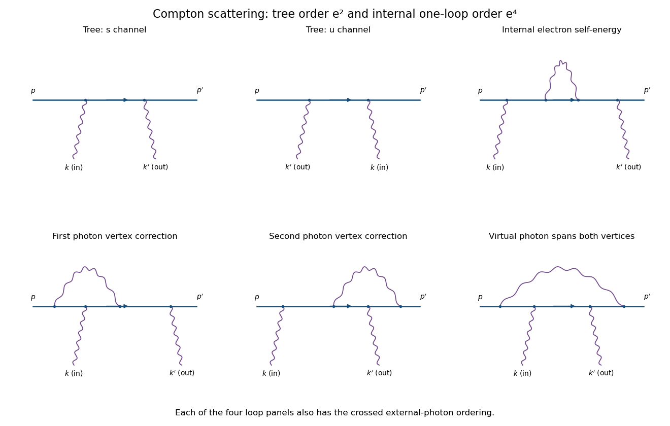
Compton tree diagrams and the four one-loop classes before exchanging the external photons
. Details. 
To prove the incoming Ward identity, replace by and write , with the Feynman boundary prescription understood. The physical nonzero-photon kinematics keeps these tree denominators off the electron pole. Sincethe external Dirac equations implyTherefore the two contracted terms are and its negative, and cancel. By linearity,This is the two-photon fermion Ward identity. An analogous cancellation holds for the outgoing photon. Gauge-equivalent polarization representatives have the same scattering amplitude, so a longitudinal pure-gauge component is not an extra physical photon state. Individual diagrams do not generally satisfy this identity; their sum does.
For perturbative order, each elementary QED vertex has one photon leg. If is the number of internal photon lines and , the vertex parity of a QED amplitude givesThus there is no third-order contribution. At fourth order, and, counting all three legs per vertex with four external legs, . A connected graph has loop number .
The nonzero one-loop classes on the open electron line are an internal-electron self-energy insertion, a vertex correction at either external-photon vertex, and a virtual photon spanning both photon vertices, giving the four-point box class. The first figure sketches each class for one photon ordering; interchange the two external photon attachments for its crossed partner. This yields two internal-self-energy graphs, four vertex graphs and two spanning-box graphs. They use the usual photon propagator, for example in Feynman gauge.
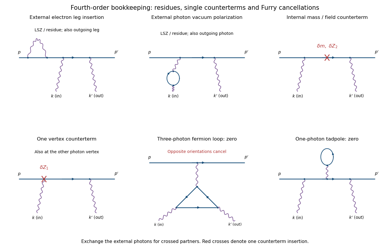
External-leg insertions, fourth-order counterterms and the odd-photon loops that cancel
. Details. 
For completeness, one-loop diagram classes for Compton scattering also depend on whether one is drawing an unamputated correlation function or a physical amplitude. Electron self-energies can be attached to either external electron leg, and photon vacuum polarization can be attached to either external photon leg, for both photon orders. In an on-shell renormalized S-matrix, these are accounted for by LSZ reduction and external-field residues rather than counted again as independent amputated graphs. Photon-leg corrections are not vacuum-polarization insertions on an internal Born photon: there is no such Born line.
At the same fourth order, a renormalized calculation has one mass or electron-field counterterm on the internal electron line, or one vertex counterterm at either Born vertex; the crossed partners are included. Each counterterm is a relative order- correction to the order- tree amplitude. External-field normalization must follow the same convention.
A possible closed electron loop with three photon vertices, linked to the external electron line by a virtual photon, cancels between its two orientations by Furry's theorem. Transposing the loop and using gives an extra sign , so its orientation-reversed partner is its negative. A one-photon tadpole likewise vanishes. Disconnected vacuum bubbles are removed by vacuum normalization. The first genuine radiative corrections are fourth order, with the internal self-energy, vertex and spanning-box classes and their consistently included renormalization terms.
Articles by others on the same topic
There are currently no matching articles.