Write for the controlled unitary gate. For a normalized eigenvector , the first Hadamard gate and quantum phase kickback giveThe final Hadamard gate therefore produces the unentangled outputThe auxiliary system is unchanged, while its eigenphase becomes accessible through interference of the control qubit. The special unitary group assumption is not needed for this calculation; unitarity and the normalized eigenvector suffice.
Apply the Born rule to the two amplitudes in the introductory calculation. In the computational basis, the probabilities areThe other basis printed in this question is , the Pauli Y gate eigenbasis. It is not the real Hadamard basis. Write the output amplitudes as and . The plus-outcome amplitude is and the minus-outcome amplitude is . Since , the Born rule givesIn particular, at the output is the minus eigenstate, which checks the sign of the imaginary quadrature.
Use separate fresh runs for each measurement basis. If denotes the empirical outcome frequency, thenThe two differences estimate and , resolving the ambiguity that would remain from the first basis alone. Each Bernoulli frequency converges by the strong law of large numbers, with standard error of order the inverse square root of the number of runs. One may project the noisy estimate onto the unit circle if a phase estimate is desired, but that projection is not necessary for consistency.
The mixed-state expression in the PDF contains a mismatched bra in its second term. A probability mixture of the stated orthonormal eigenvectors must be interpreted as . Taken literally with a different bra, it need not be Hermitian or positive and is not generally a density operator.
Let . A quantum channel and its measurement probabilities are linear in the density operator, so averaging the pure-state results givesTherefore the same frequency estimator yieldsMore generally, after the controlled operation and before the final Hadamard gate, the reduced control density operator isThis follows by a partial trace of the control blocks , , and . It proves the mixed-state Hadamard-test quadratures for any auxiliary density operator, even one not diagonal in the eigenbasis. Conjugation by the final Hadamard gate maps to and to , explaining the imaginary-part sign.
Prepare the auxiliary system in the maximally mixed state . Then , so the two measurement bases giveThere is no need to know the eigenvectors of . Choose a uniformly random member of any known orthonormal basis on each run; discarding the classical preparation label produces . Alternatively, discard one half of a maximally entangled pair of -level systems. This is trace estimation by a maximally mixed Hadamard test.
The circuit directly estimates the normalized trace. To demand fixed absolute accuracy in the unnormalized trace requires normalized accuracy ; straightforward independent frequency sampling consequently uses order runs at fixed confidence. Thus the construction should not be confused with a dimension-independent guarantee for arbitrary absolute trace precision.
Apply one Hadamard gate independently to each qubit. These gates act in parallel, so the quantum circuit implements with gates and depth one.
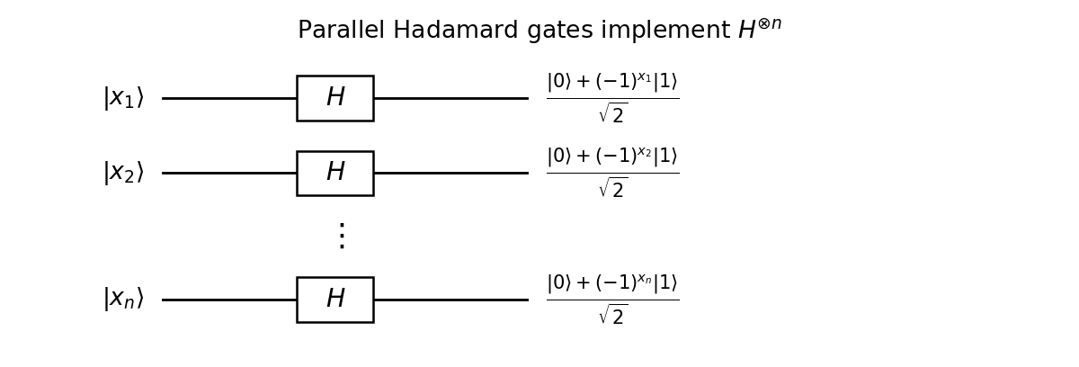
Parallel Hadamard gates implementing the binary Fourier transform
. Details. 
For a computational basis state, factorization givesThe exponent is the dot product over the finite field , because multiplying the separate signs adds their exponents modulo two. This is the Walsh-Hadamard transform, equivalently the quantum Fourier transform on the finite Abelian group .
In particular, the all-zero input becomes the uniform coherent superposition . It is a useful initial operation because an oracle can then act on all amplitudes in one call, and subsequent interference can reveal a global property. Measurement alone does not read all function values: the later interference step is what turns the preparation into an algorithmic advantage.
The first Hadamard transform prepares a uniform superposition in the first register while the second stays zero. The Boolean quantum oracle, now with an -bit output register and bitwise addition, therefore givesThis state is normalized because distinct labels are orthogonal, even when their oracle outputs coincide. Addition in the oracle is bitwise exclusive-or, making the oracle reversible; replacing the first register by would not define a unitary gate for a two-to-one function.
For the later recovery steps we use the intended nonzero hidden-period promise . Then two-to-one behavior and force each fibre to be exactly . The printed allowance does not explicitly exclude zero. If zero were allowed without a nonzero-period promise, the displayed identity would hold trivially for every function and would not specify Simon's problem. That distinction is addressed again in the query count.
Only strings in the image of can be observed. Choose one preimage of an observed string. Under the nonzero-period promise its two preimages are and . The Born rule gives probability to this second-register outcome, and conditional normalization leaves the first-register coset stateThe relative plus sign is retained: measuring the output register reveals which fibre was sampled but does not reveal which member of the fibre was present. Measuring its bits successively gives the same projection onto the observed full string as measuring the whole register at once.
Apply the Hadamard transform to the conditional coset state. The amplitude of a first-register output isWhen over , the two terms cancel exactly. When , their squared modulus is . ThusThere are orthogonal outputs, so these probabilities sum to one. The distribution is independent of the particular observed fibre. It is the Single-sample distribution in Simon's algorithm: each run gives a uniform random equation restricting the hidden period to the orthogonal complement over the binary field.
Each independent run uses one oracle call and gives a uniformly sampled equation . Collect linearly independent equations and use Gaussian elimination over . Their solution space has dimension one and consists of , so the promised nonzero solution identifies uniquely.
To quantify the expected query count for Simon sampling, write . If the existing equations have rank , their span contains of the possible samples. A fresh equation raises the rank with probability . The mean waiting time is the corresponding geometric distribution mean, givingThe last sum is less than : its first term is and its remaining terms are bounded by . Hence the expected number of quantum queries is . For a fixed high-confidence budget, use samples. Failure to span means that a nonzero linear functional on the -dimensional sampling space annihilates every sample. Each such functional has probability , so the union bound gives failure probability at most . Thus queries suffice for failure probability at most . For , the nonzero string is known already and no samples are needed.
Classically, a collision between distinct queried arguments immediately yields . Random queries produce this collision after order calls, by the birthday problem. Conversely, choose the nonzero period uniformly and label the fibres randomly. Before a collision, queries can exclude at most periods, their pairwise argument differences; every remaining period has the same no-collision transcript distribution. When , those exclusions occupy a vanishing fraction of the candidate periods, and neither collision discovery nor guessing a remaining period has a constant success probability. More quantitatively, conditioned on no previous collision, the next query tests at most of at least remaining periods; summing these conditional probabilities proves the same square-root lower bound. Therefore the optimal bounded-error classical query count is , exponentially larger in than the quantum count.
This comparison presumes a hidden nonzero period. Under a literal interpretation asking merely for some satisfying the printed identity, returning requires no queries at all, quantum or classical. Nonzero is the necessary intended promise, not a consequence of two-to-one behavior alone.
Let . The joint state after the environment interaction is . Taking its partial trace over the environment gives the exact reduced density operatorThe conjugate in the upper off-diagonal entry follows from tracing . Normalization of the environment states and the Cauchy-Schwarz inequality imply .
For comparison, a phase-flip channel sends to , multiplying its off-diagonal entries by the real number . Consequently the claimed representation is valid, for a general input, provided the environment overlap is real, withThis is a genuine probability between zero and one. The environment maps printed in the question do not themselves imply that is real. For example, choose , so , and take . The qubit becomes , whose imaginary off-diagonal entries cannot come from any probabilistic mixture of and . These environment maps are a valid isometry and can be extended to a unitary interaction, so this is an actual counterexample to the unrestricted premise.
The general complex environment overlap in qubit dephasing has an exact corrected description. Write , , and let . ThenAt , choose any phase. The dephasing channel includes both random phase errors and, when the overlap is complex, a coherent diagonal rotation. The subsequent probability formulas use the intended real-overlap phase-flip model.
Subtract the two density operators. The difference is Hermitian with zero diagonal and off-diagonal entry . A matrix has eigenvalues , because its square is . Its two singular values are therefore both . By the definition of the trace norm,For the intended real-overlap phase-flip channel, , givingThis vanishes for a computational basis state, since a phase flip then changes only an unobservable global phase. Its largest value at fixed is , attained when . The general formula remains correct even when the probabilistic premise of part 1 fails.
Assume the three physical phase-flip channels act independently, with the same probability on each qubit, and encoding, recovery and decoding are ideal. Zero or one physical error is corrected. HenceThe probability of an uncorrectable two- or three-site error is .
One must also choose the logical convention consistently with the output phase error specified here. The usual phase-flip repetition code with codewords and has residual operator after two or three physical errors: their error syndrome equals that of the complementary zero- or one-error pattern. This operator exchanges those codewords, so plain inverse encoding would give logical , not .
To obtain the stated logical phase-flip convention, use the logical Hadamard convention for a phase-flip repetition code. Put a logical Hadamard gate before that encoding and after its decoding. The encoded state iswhere the plus and minus states in these codewords are the real Hadamard basis states. The uncorrectable exchange is now conjugated to . With that convention the decoded density operator and its trace distance are exactlyFor , , so coding reduces the trace distance. The displayed recovery probability means success of correction as a quantum operation on an arbitrary unknown input. If the particular input is a eigenstate, even the logical phase-error branch represents the same physical state, and the probability of recovering that particular state is one.
Independence is an extra noise assumption needed for the numerical probability. If all three physical qubits flip together with probability , each marginal still has the given phase-flip channel, but the logical failure probability is , not . More generally, for a classical joint phase-error distribution with a random number of flips, and ; the same decoded mixture holds in the stated logical convention. Thus marginal error probabilities alone do not determine the requested recovery probability. A complex environment overlap likewise requires the coherent rotation to be retained or separately compensated before this stochastic phase-error analysis applies.
For independent attempts, measuring after each application of produces a success with probability . Recognize the answer with the verifier and restart on failure. The number of attempts has a geometric distribution, with . Summing the tail probabilities givesThis counts applications of ; it presumes and a fresh preparation for each attempt. If , neither repetition nor the amplification construction can create a good component from this input.
Let project onto the good-output subspace and let , . They are orthonormal because their supporting computational basis strings are disjoint. The verification unitary operator is , so and .
Also . Since , conjugating gives . ThusBoth reflections preserve the span of and : is diagonal there, and the other reflection only adds a multiple of , already in that span. Direct substitution of yieldsThe minus sign in the first image follows from applying before the state reflection. In the ordered basis the matrix isThis exhibits the invariant plane without assumptions about the action of on the other input basis vectors.
Choose with . Then and . The matrix found in part 2 is a rotation by in the ordered good-bad plane, with the bad coordinate listed first. The initial coordinate vector is .
After rotations its angle from the bad axis is . Equivalently, multiplication of the displayed matrix and the addition formulas for sine and cosine prove the assertion by induction from . HenceThe Born rule therefore gives good-output probability . This is the geometric mechanism of amplitude amplification: each coherent iteration rotates the already existing good amplitude toward the good axis.
For known , use nearest-integer stopping for amplitude amplification. SetWriting , the difference between and has absolute value at most . Thus . The Born rule and part 3 giveCount the initial once and the and occurring inside each of the amplification iterates. The number of applications of either preparation unitary is thereforeThe counts separately are applications of and applications of , in addition to applications each of and . This is a quadratic improvement over the mean number of unamplified trials. At an exact rounding tie either nearest iterate meets the probability bound. Knowledge of is used in selecting the stopping time; repeatedly applying without a suitable stopping rule can rotate the state past the good axis and reduce success again. The fact that answers lie in NP supplies verification, but by itself gives no claim that is polynomial in input length.
Articles by others on the same topic
There are currently no matching articles.