The normalized timelike normal has . Multiplying the linear projections givesAlso . ThusThe operator fixes every vector tangent to the spacelike hypersurface and annihilates its normal. The repeated-index typo in the TeX is resolved by the actual PDF's matrix-composition indices.
Use metric compatibility and differentiate the projector:Projecting the derivative and lower tensor index kills the first term, by part (a). The remaining term is the extrinsic curvature:The second projection may be inserted in the definition of , since differentiating gives .
For a tangential covector, the projected derivative is . Its second derivative isExpanding by the product rule, the derivative of the first inner projector gives . This contribution cancels on antisymmetrizing , because is symmetric.
The derivative of the second inner projector gives . Differentiating tangentiality, , rewrites it asThe remaining term is the projected four-dimensional curvature commutator. Using the curvature convention of the question,and replacing the tangential by , we obtainSince this holds for every tangential covector, the Gauss equation follows:The signs use a timelike unit normal and the specified commutator convention; reversing a curvature convention without changing the commutator would change the comparison.
For a homogeneous canonical massless scalar field, the flat Friedmann equation and field equation in conformal time arePut . On the negative-time branch, , and . ThereforeBoth equations are satisfied. Since , this is cosmological contraction with a free homogeneous scalar. Its energy density and pressure are equal, so it is a stiff fluid, and the scale factor tends to zero as .
The massless scalar stress tensor in mixed-index form isIn conformal Newtonian gauge, and to first order. Spatial gradients of the background vanish, so products of two spatial perturbation gradients are second order. ConsequentlySubstitution yieldsThe potential multiplies only second-order gradient products in these components. The same reasoning makes the off-diagonal spatial stress vanish at first order, consistent with .
Let . The momentum constraint gives . Differentiating it and using the background field equation givesInsert this into the energy constraint, whose right-hand side in the PDF contains :Rearranging and expanding givesHere and . The coefficient of cancels, provingThis also identifies the derivative lost from the background-field square in the TeX transcription.
For each Fourier mode the equation is . Set . Direct differentiation removes the first derivative and givesFor , the inverse-square term is negligible, and the positive incoming-frequency branch has . ThereforeThe momentum constraint then giveswhere . Thus the scalar perturbation has precisely the required behavior. Conversely, the two constraints imply the potential equation in part (c); reconstructing by the momentum constraint therefore satisfies the energy constraint too. This checks compatibility beyond simply comparing powers of .
For the exact mode equation write and . Substitution givesThe positive incoming-frequency solution is the Newtonian-potential Hankel modes in stiff contraction branchFor large , . Part (d) and the normalized scalar incoming mode giveAt late times, , so the leading growing cosmological Newtonian potential is . Hence the vacuum-normalized Newtonian spectrum in stiff contraction isFourier-volume conventions can modify the overall normalization but not this exponent. The dimensionless power per logarithmic interval is , corresponding to if written as . The question asks the dimensional mode variance's exponent, which is ; it is also important not to substitute a curvature-perturbation spectrum for the specified cosmological Newtonian potential.
Use the comoving cold dark matter choice in synchronous gauge. Its continuity equation gives . Substituting and into the metric tensor equation yieldsFor radiation, put . The continuity and Euler equations become and . Differentiating the first and eliminating the other two variables givesThe radiation sound speed is .
During radiation domination, , and . Outside the horizon, , the gradient term is negligible. The regular initially adiabatic mode has to leading order. Consequentlywith powers and . Keeping the regular growing branch givesThe superhorizon density contrasts here are in the specified comoving synchronous gauge; density contrast is not a gauge-independent superhorizon observable.
Deep inside the horizon, still before equality, radiation pressure produces bounded acoustic oscillations at frequency . The leading form isTo see the logarithmic growth, average the rapidly oscillating radiation forcing in the Cold dark matter equation and neglect the small matter self-gravity term; the remaining equation is . Radiation does not have a secular growing acoustic amplitude in this approximation. Its source supplies only a smaller slowly varying response, asymptotically , while the radiation oscillations induce suppressed oscillatory corrections to Cold dark matter.
The matching can be made explicit in the leading system. Put and defineEliminating radiation gives . Direct differentiation verifies that the regular adiabatic solution isIndeed at zero, and the radiation bracket is , recovering the early amplitudes. At infinity, and . This adiabatic radiation-era cold-dark-matter transfer solution fixes the logarithmic coefficient and leading acoustic phase rather than leaving matching arbitrary.
The constants and acoustic phase are fixed by matching through horizon entry, not by imposing the early adiabatic relation at every later time. Since entry occurs at , their amplitude scale is set by . This is the Mészáros effect: logarithmic subhorizon Cold dark matter growth accompanies radiation oscillations until matter becomes dynamically important. Factors such as in defining a wavelength do not change the two asymptotic regimes.
Continue to choose the CDM-comoving synchronous frame. For nonrelativistic baryons, neglect corrections to gravitational density weights and Hubble friction, but retain , since gradients may compensate its small coefficient. ThenTogether with the metric tensor equation these giveThe friction terms contain first derivatives, as the original PDF confirms; they are missing in the TeX's transcription of these equations.
When , Cold dark matter sets the gravitational forcing. Its matter-era growing mode is . Compare pressure with the gravitational timescale:Converting the comoving wavenumber to a physical wavelength givesFor , pressure is negligible and baryons can follow the growing Cold dark matter mode. In that limit subtracting the two equations gives for , so . Relative to , this offset vanishes: baryons catch up.
The phrase “only grow” needs this gravitational-growth interpretation. For a small baryon fraction the baryon equation is forced, not an autonomous Jeans-instability equation. At , its slowly varying response isplus acoustic transients. It is suppressed rather than identically absent. For example, with constant sound speed, and , the equation is . Its particular solution is constant, and its oscillatory homogeneous part decays as . This demonstrates Jeans support versus forced baryon response; the scale above is not a theorem forbidding every forced or transient sub-Jeans change.
Before decoupling, tight photon coupling makes the effective sound speed large, about . The small- approximation just derived is not quantitative in that regime; the coupled photon-baryon fluid must be used. Its large pressure supports acoustic oscillations, and baryon clustering below the corresponding large Jeans/sound scale is inhibited while Cold dark matter wells grow. After decoupling the supplied sound speed is tiny and decreases further as the gas cools. The Jeans length drops sharply, so many previously supported modes fall into Cold dark matter wells and approach its growing density contrast. Modes still below the instantaneous pressure-support scale remain suppressed. The subsequent detailed thermal scaling depends on the gas's temperature evolution; the given sound-speed history suffices for this qualitative conclusion.
Let . A comoving observer measures photon energy , so . The null condition is . Using the stated Christoffel symbols in the time geodesic equation givesDivide by to differentiate with respect to conformal time. The background redshift term cancels when differentiating :In the perturbation term use the background relation , givingWithout metric tensor perturbations, both and the propagation direction are constant along an unperturbed ray. Thus and are first order. Multiplying them by derivatives of , which is also first order, gives second-order terms. The term is first order and must be retained. At linear order the Collisionless Boltzmann equation therefore readsTaking the Fourier transform in the spatial coordinates provesA first-order correction to the propagation velocity multiplying a spatial derivative of is likewise second order.
Write , with at linear order. Since , the background Planck function depends only on comoving momentum. Expanding its temperature-shifted argument givesUsing rather than in the perturbation denominator changes only higher-order terms.
The photon brightness perturbation is the energy-weighted angular perturbationIntegration by parts gives ; the boundary term vanishes at both endpoints for a Planck spectrum. Therefore . Multiplying the transport equation by and integrating yields the synchronous photon brightness equationThe PDF's definition is ; the TeX's denominator is a transcription error.
Expand in Legendre moments in . The monopole is the density/temperature perturbation, and the dipole is the bulk velocity. Before decoupling, rapid Thomson scattering isotropizes photons in the electron rest frame. In the tight-coupling approximation, the scattering rate is much larger than and , so the quadrupole and higher moments are suppressed by the mean-free-path parameter, with the quadrupole typically of order times the dipole. To leading order only monopole and dipole are needed. This suppression uses the collision term restored before decoupling; it does not follow from the collisionless equation by itself. Finite quadrupole corrections generate polarization and diffusion damping.
The emission-density term is the intrinsic temperature fluctuation: blackbody radiation has , hence the factor . Adiabatic compression and rarefaction of the photon-baryon fluid create coherent density extrema at last scattering. Their projection produces acoustic peaks, with angular scale set by the sound horizon divided by the distance to last scattering. In a familiar nearly flat cosmology the first prominent temperature peak is around degree scales, of order a few hundred; precise positions depend on the background.
The velocity term is a Doppler effect from the emitting plasma's line-of-sight motion. The acoustic velocity is approximately a quarter-cycle out of phase with the density oscillation. Its projected contribution is strongest on acoustic and smaller angular scales and interleaves with density extrema, with projection broadening its features. Both sources are suppressed on sufficiently small scales by Silk damping and the finite thickness of last scattering.
The metric tensor integral describes photon-energy shifts during propagation through the changing perturbed geometry. In synchronous coordinates its split from the intrinsic endpoint term is gauge dependent. Rewriting the observable in Newtonian variables produces the usual emission Sachs-Wolfe effect and the Integrated Sachs-Wolfe effect from evolving potentials, with the appropriate endpoint terms. The ordinary large-scale Sachs-Wolfe combination gives a low-multipole plateau for nearly scale-invariant initial curvature power. Late-time evolving potentials chiefly affect large angles, often ; evolution near radiation-matter equality also drives an early integrated contribution near the first acoustic peak. Static matter-era potentials do not produce that Newtonian integrated contribution.
All emission quantities are evaluated at the last-scattering endpoint and the metric tensor source along the unperturbed photon ray, not at a single fixed spatial point throughout the integral. Observer monopole/dipole conventions do not change this physical interpretation.
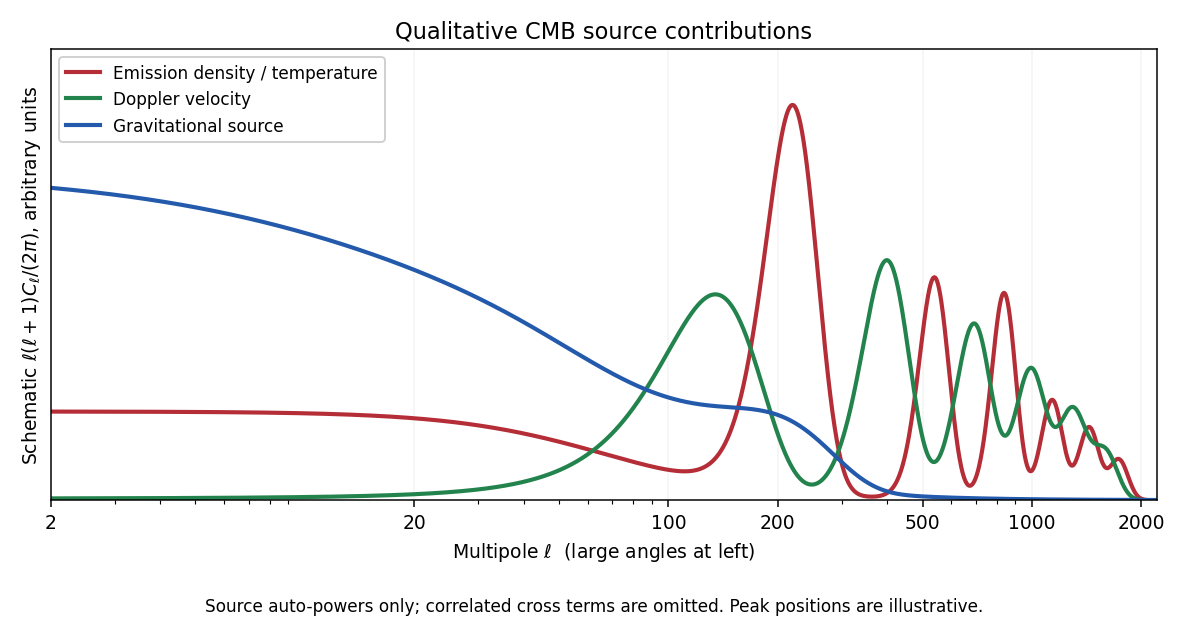
Schematic density, Doppler and gravitational contributions to CMB angular power, with correlated cross terms omitted
. Details. 
The sketch uses arbitrary units and representative scales. It displays source auto-power shapes, not measured data or an assertion that the total power is their simple sum. The terms are correlated; their cross-power contributions and the gauge-consistent endpoint combination are essential in an actual angular-spectrum calculation.
Printed metric tensor. There is a genuine false premise. For the metric tensor actually printed, introduce . Since and ranges over all real values,This is global two-dimensional Minkowski spacetime, an example of how a time-dependent lapse can disguise flat spacetime. A future-directed timelike geodesic from the stated event, parametrized by proper time , hasFor the spatial position is unbounded, not periodic; is strictly increasing. The curve , is an explicit counterexample. Physically these are inertial particles moving at constant Minkowski velocity . The nonlinear original time coordinate does not create a confining force.
Likely intended spatial lapse. The hint instead fits the different metric tensor , the unit-radius two-dimensional anti-de Sitter spacetime in global static coordinates. This interpretation is not substituted silently for the printed one. For that metric tensor the conserved energy is , and normalization givesPutting gives , hence an outgoing geodesic from the origin hasThe supplied integral shows that increases by over each proper-time half-period. Thus the spatial oscillation repeats after proper time and coordinate time , with turning points . It describes gravitationally confined inertial motion in AdS. On the universal cover, is not identified and the worldline is not closed; identifying modulo makes the timelike geodesic closed. For the central particle stays at .
For the printed metric tensor, first use the global Minkowski time . SetThenRemoving the positive conformal factor yields the ordinary Penrose diagram of two-dimensional Minkowski spacetime: a diamond with null future/past infinity on its sloping edges, timelike infinity at the top/bottom, and spatial infinity at the left/right corners. Null geodesics have slope ; future/past causal cones are ordinary Minkowski cones. There is no physical boundary or curvature singularity at a finite original coordinate value.
For the alternative spatial-lapse metric tensor identified in part (a), set . Then and , soIts universal-cover conformal diagram is an infinitely tall strip with two timelike conformal boundaries, the conformal strip of two-dimensional anti-de Sitter spacetime. Null geodesics reach either boundary in finite coordinate time, though the boundary is not part of the physical manifold and the physical null affine parameter diverges there. The strip and diamond have different causal structures; no conformal coordinate change can identify their global causal properties.
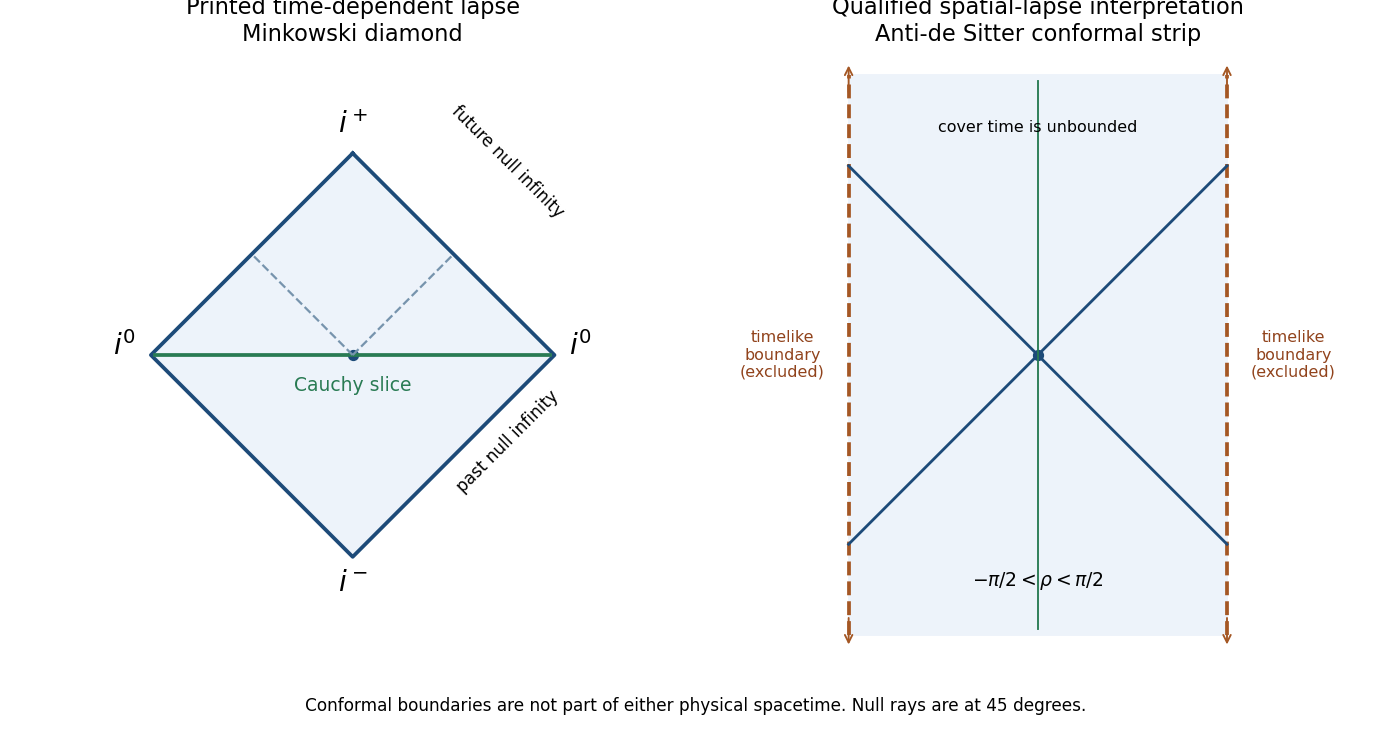
The Minkowski diamond for the printed time-dependent lapse and the AdS conformal strip for the explicitly qualified spatial-lapse interpretation
. Details. 
For the printed spacetime, yes. The surfaces , equivalently , are Cauchy surfaces in Minkowski spacetime. Every inextendible causal curve intersects each once; if its monotone time coordinate had a finite endpoint, the bound would give a finite spatial endpoint too, allowing continuation. Causal diamonds are closed and bounded in and hence compact. Therefore the printed spacetime is globally hyperbolic.
Initial data on a Cauchy slice determine unique causal evolution for the usual well-posed hyperbolic field equations, without boundary data at spatial infinity at finite time. The time reparametrization preserves that property.
For the qualified AdS interpretation, no. On the universal cover, choose two central events with enough time separation for a null ray to approach a strip edge and return. Their causal diamond contains a sequence with but no limit in the physical spacetime, so it is noncompact. A constant- surface fails to meet every inextendible causal curve arriving from timelike conformal infinity. Thus even the cover is not globally hyperbolic. Field evolution needs appropriate boundary conditions, such as a reflecting condition compatible with the field theory, as well as initial data. If AdS time itself is periodically identified, closed timelike curves give an additional and more immediate obstruction. These are consequences of the alternative spatial-lapse geometry, not of the printed flat metric tensor.
Let denote geodesic distance from the charge; is the fixed curvature radius, not the radial variable. In round three-dimensional hyperbolic space, a sphere has areaUsing the convention that electric flux is , Gauss's law gives the radial orthonormal electric fieldIts magnitude is , and a negative charge reverses the direction. In rationalized natural units set ; Gaussian conventions instead use flux .
For this approaches . For , . This hyperbolic-space Coulomb field falls rapidly because the sphere area grows exponentially; conserved electric flux is unchanged. A potential vanishing at infinity is .
The original PDF actually prints rather than in the angular metric tensor. The round angular factor used above is required by its description as hyperbolic space. If the printed angular metric tensor is taken literally, the sphere-area coefficient is insteadand a radial Gauss-law solution has . That angular geometry is not a smooth round sphere, so the literal metric tensor does not describe the asserted homogeneous hyperbolic space. Both readings retain the same radial area-growth factor; the geometric repair is explicit.
Define , in the three noncompact spatial directions, and . The compact source must be the periodic Dirac deltaFor the wave operator as explicitly defined in the question, a retarded circle-compactified massless propagator isThe poles are both below the real axis, making the integral vanish for . Performing just the frequency integral gives an equivalent expressionThe first time derivative of jumps by one at zero, so applying yields . Together with the completeness relations for the Fourier series and Fourier transform this verifies the specified source and normalization. The symbol for the wave operator follows the question's explicit sign convention; it is the negative of for its mostly-plus metric tensor.
Each compact Fourier mode obeys the noncompact equation with dispersion relation , whereThus momentum in the extra dimension appears as rest mass to a four-dimensional observer. There is one massless zero mode and equally massive modes. For a real scalar they can be organized into sine and cosine components rather than independent complex fields.
At equal compact positions all phase factors are one, and the propagator becomes the Kaluza-Klein towerThe factor follows from the normalized compact eigenfunctions. It cannot be discarded if the five-dimensional field and source normalizations are retained.
At distances and elapsed times much smaller than , propagation probes the local covering space and resolves the compact direction. Formally becomes when many nearby compact momenta participate, giving the massless five-dimensional retarded Green function. Equivalently, the compact Green function is a sum of covering-space images at . Before a signal can travel to any nonzero winding image, only the direct image contributes. Short-scale physics is five-dimensional.
At low frequency and long wavelength, , massive modes cannot be excited as propagating particles, and the massless zero mode dominates at long noncompact range. Then , with higher-mode corrections and the corresponding effective source normalization. Low-energy long-scale physics is four-dimensional.
A precise static illustration avoids ambiguities of pointlike retarded signals. At equal compact positions and zero frequency, the Yukawa potential sum isThis static Green function across a circle compactification has limitsThey are the Coulomb kernels in four and three spatial dimensions respectively, with exponentially small massive corrections at large .
For an unsmeared point-source retarded distribution, coordinate separations alone are not enough to impose a low-energy approximation. A high-frequency pulse can still excite massive modes and resolve winding signals at arbitrarily long travel distance/time; its image fronts satisfy . Thus large separation does not impose a Kaluza-Klein low-energy limit. The usual large-separation four-dimensional statement means low-energy sources or coarse-grained measurements, or a static long-distance limit. It is not a universal pointwise limit erasing all massive oscillations from a sharply resolved retarded pulse.
Articles by others on the same topic
There are currently no matching articles.