The Hamiltonian functional isTreating the field and its complex conjugate as independent variables, and integrating the gradient term by parts with periodic, decaying or fixed-field boundary conditions, givesThus is the Gross–Pitaevskii equation. The factor in the interaction energy avoids counting each pair twice.
At prescribed particle number, minimize subject to . Introducing the chemical potential as a Lagrange multiplier, the variation of vanishes at a ground-state profile , provingThe corresponding time-dependent field is . A solution of this stationary equation is only a candidate ground state; the ground state is the minimizer among all fields satisfying the normalization. For the uniform repulsive gas in a periodic volume, the gradient energy is nonnegative and , so the constant-density, constant-phase state is indeed the minimum. The uniform-background solutions below assume and a positive background density.
Let the uniform background number density be and set . The subtraction of this chemical potential requires a phase rotation as well as a rescaling:Substitution into the physical Gross–Pitaevskii equation givesConsequently the requested coefficients follow fromThe length unit is the specified healing length. Removing tildes produces the paper's dimensionless equation; in particular the coefficient of its time derivative fixes , not its reciprocal. Without the phase rotation the linear term would not appear.
The dimensionless ground state is for any constant phase , conventionally . Its subtracted energy is proportional to , which is nonnegative and vanishes for this state. In physical variables it has density and phase rotating at .
Use translating coordinates and a profile ; the background condensate remains at rest in the laboratory. Then , and the Gross–Pitaevskii solitary wave equation isThis is a coordinate translation of a traveling solution, rather than an additional phase boost to change the background flow.
Set with small real . Since , the real and imaginary linearized equations areFor a longitudinal sinusoid, choose and . Their coefficients obeyA nonzero solution therefore requires , giving the positive-direction phase velocityEquivalently the time-dependent linear Bogoliubov spectrum is and . Its long-wavelength sound speed is , which becomes in physical units using . For a general wavevector , the stationary resonance is ; specifying only its magnitude does not determine the velocity unless its direction is also fixed. This sinusoidal dispersion describes linear radiation about the background, not an amplitude-independent dispersion law for every nonlinear solitary wave; localized subsonic waves do not require a real oscillatory far-field wavenumber.
For a straight unit-winding quantum vortex, the real radial amplitude satisfiesIn the frame translating with the ring, put and , where is independent of the angular coordinate. The cylindrical Laplacian has the exact identityAfter inserting this into the translating Gross–Pitaevskii equation, subtract the straight-vortex equation. Because is real,and direct expansion of the nonlinear difference givesThus the exact ring-on-line perturbation equation, including its quadratic and cubic terms, isThe two appearances of are responsible for the coefficient multiplying inside the bracket. No small-amplitude approximation is needed for this identity.
The single-particle Hamiltonian has a periodic potential . Define the unitary spatial translation operator . Its derivatives commute with translation, and the potential's periodicity gives .
Each energy eigenspace is therefore preserved by , so within it one may choose simultaneous energy and translation eigenstates. On a large periodic interval of cells, and its eigenvalues are phases , with ; the infinite-volume limit gives continuous quasimomentum modulo . For a simultaneous state in band , this provesThen obeys , which constructs the usual Bloch state rather than assuming its form. The label distinguishes energy bands at the same crystal momentum . In a degenerate energy eigenspace an arbitrary superposition need not itself have one translation phase; the result refers to the simultaneous Bloch states.
Let be the normalized stationary profile. Multiplying its stationary Gross–Pitaevskii equation by , integrating and integrating the kinetic term by parts yieldsThis is not simply : the quartic contribution is twice its contribution to that energy per particle. For an infinite periodic system one uses one cell and the corresponding cell particle number, or equivalently average densities.
At fixed lattice spacing, mean density , coupling and temperature, the commonly used condensate compressibility in an optical lattice isIf compressibility means the thermodynamic volume response instead, the Gibbs-Duhem equation at zero temperature gives . Stating the convention removes this factor-of-density ambiguity; the lattice-depth derivative has the same sign at fixed .
For the stable repulsive ground-band Bose-Einstein condensate, the intended trend is for increasing nonzero lattice depth, with mean density held fixed. Deeper wells localize the field, enhancing the repulsive interaction response. To quantify this, in the weak-interaction band approximation write , with the cell average of equal to one. Perturbation in givesIn deep wells the localized orbital is approximately a normalized Gaussian of width . Neglecting interwell overlap, , hence . This explicitly establishes the sign in that controlled regime; the repulsive ground-band calculation describes the broader trend.
The sign statement needs the repulsive, stable ground-band interpretation, not merely the literal assumption . It also need not be a strictly nonzero derivative at : at weak interaction , with normalization corrected at second order, gives and a zero initial slope. A leading density-dominated Thomas–Fermi approximation for a condensate with density positive everywhere gives and no depth dependence of this response at that approximation's order. These limits do not justify a strict universal sign for every unspecified interaction and parameter regime.
Use the stationary quantum vortex fieldwith no dependence on the coordinate along the vortex line. The polar Laplacian contributes . ConsequentlyA regular vortex with nonzero integer winding number has near the origin. The angular phase gives the superfluid velocity outside the core. For , the exterior amplitude responds to the periodically varying potential; it is not generally a constant bulk value. The radial potential here is not a Cartesian translation-invariant optical lattice, so the Cartesian Bloch theorem is not an exact theorem for its full radial equation.
Set , , using the healing length and . For zero external potential, division by producesPrimes now denote dimensionless-radius derivatives. Let . Then , while the centrifugal term is and . Their leading balance gives . Therefore the inverse-square tail of a Gross–Pitaevskii vortex yieldsFor a singly quantized vortex the answer is . This is the amplitude deficit; the density deficit has limiting coefficient instead.
A nonzero radial lattice prevents a unique universal curve without values of the depth, period, chemical potential, coupling and winding number. An explicit example of the requested profile is shown below for , repulsive coupling, and ; since , this corresponds to .
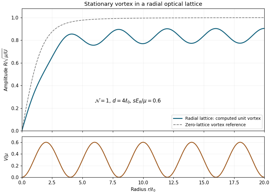
Computed unit-vortex amplitude in a radial optical lattice, with the lattice potential and homogeneous-vortex reference
. Details. 
The plotted dimensionless amplitude is . The generator solves the nonlinear radial equationby finite differences and damped Newton iteration; here is in healing length units. It imposes regularity and a zero radial derivative at , well outside the plotted interval . The exterior boundary is at a potential minimum, and its placement is checked by an extended-domain calculation.
The quantum vortex core still forces the amplitude to vanish at the origin. Farther out, amplitude minima occur near potential maxima, where repulsion and trapping reduce the local equilibrium density, and amplitude maxima occur near the low-potential annuli. Gradient energy smooths the modulation, so the profile does not exactly follow the local estimate . It approaches a periodically modulated exterior background rather than the homogeneous limit one; the dashed zero-lattice curve is included solely as a reference. At sufficiently deep lattice barriers the density troughs can become much more pronounced than in this example.
Take , with the same time coordinate in both frames. The normal fluid transforms as . The field transformation is the unit-modulus Schrödinger boostWriting the phase as makes differentiation at fixed primed position transparent:It follows that both and gain the same terms . The density is unchanged, , so the nonlinear local term has the same form.
The remaining material derivative transforms asThus the density-damping term acquires only the common phase factor, proving invariance of the complete equation under a Galilean boost. Keeping the normal velocity unchanged in both frames would fail this check; the reference flow must transform along with the condensate.
Choose the amplitude real and positive locally, absorbing its phase into , and work away from vortex cores or other density zeros. Put and . Direct separation of the real and imaginary parts of the Gross–Pitaevskii equation gives the exact Madelung equationsFor example, the imaginary part is , which proves the density equation after multiplication by . The real damping coefficient affects the phase balance rather than adding a particle source.
Using this continuity equation and ,Taking a gradient of the phase equation gives the exact velocity equationNow , , and is order one. The inertial and chemical-potential gradients are ; the double-gradient bulk term is ; and the quantum potential force contains three slow derivatives and is , provided stays bounded away from zero. Through order this proves the requested bulk-viscous limit of a material-density-damped condensate withAdding a spatially constant value to does not affect the equation, so is an equivalent convention. The density and viscosity coefficients are in the equation's dimensionless units. The bulk viscosity term is the gradient of the divergence of the relative mass flux, not a shear-viscosity term. At density zeros the slow-amplitude expansion and the division by fail; there one must retain the original field equation.
A constant-amplitude plane wave has no density derivative and therefore no damping. The complete family iswith arbitrary constant phase . The background in the question is the member .
Use the exact amplitude–phase equations derived above with . To first order in the perturbation, and , soThese equations retain the quantum potential contribution because no long-wavelength truncation is assumed in this subpart. In particular damping contains , not the advective derivative along the moving condensate: its reference is the stationary normal fluid.
For the proposed periodic perturbation, write and . The amplitude coefficients satisfyA nonzero perturbation therefore requires the plane-wave dispersion of a material-density-damped condensateor equivalently . At zero background flow the roots are , whose real parts are negative for . As , recovers the advected Bogoliubov spectrum with long-wavelength sound speed one in these units. This differs from question 1's time normalization, whose sound speed is .
Since each species number is separately conserved, minimize with two independent Lagrange multipliers. Variation with respect to each complex-conjugate field, with boundary terms removed, givesThese are the two stationary Gross–Pitaevskii equations; the time-dependent equilibrium fields are . The cross term contributes to each equation, with no factor two, while differentiating the self-interaction term cancels its factor . Separate number conservation does not require the two chemical potentials to be equal.
For an occupied uniform two-component Bose-Einstein condensate, the gradient and trapping terms vanish. Dividing each stationary equation by its nonzero field givesThe same relations follow by differentiating the uniform interaction-energy density with respect to each number density. When , the inverse relations areThese describe a genuinely overlapping mixture only when both densities are nonnegative. An unoccupied component cannot be divided out of its stationary field equation; it requires the appropriate constrained equilibrium condition instead.
At fixed particle numbers, the perturbations satisfy . Expanding the uniform interaction energy, its linear term is , and its exact quadratic change in this contact-interaction approximation isCompleting the square givesHence the miscibility criterion for a two-component condensate isThese are precisely strict positive definiteness of the interaction matrix, and make every nonzero admissible long-wavelength density perturbation cost energy. With both equilibrium densities positive, a negative eigenvalue would instead allow a small sinusoidal perturbation along its eigenvector, with zero mean and negative energy change. The omitted positive gradient term cannot cure arbitrarily long wavelengths in an unbounded system.
If cross-repulsion exceeds the geometric mean of the self-repulsions, the unstable direction favors separation of species; sufficiently strong cross-attraction favors a joint density increase and collapse. Equality gives a zero-cost direction at this order, so it is marginal rather than strictly stable. Constraints near an absent component or finite-system wavelength restrictions require a separate boundary analysis.
Set , so , and . In the overlap region, the Thomas–Fermi approximation for a condensate neglects the gradient terms and requiresInverting this matrix proves the unambiguous profilesUsing and introducingthese Thomas–Fermi profiles for unequal condensate trap curvatures becomeThere is a genuine printed error: the PDF puts rather than in the second bracket as well. In the first bracket its coefficient requires , while in the second it requires ; for nonzero cross-coupling these cannot both hold unless the curvatures are equal. The TeX additionally drops both occurrences of . The matrix-inverse formulas above give the corrected general answer directly.
For example, , , , , give the physical overlap profiles , . Using in both printed brackets would instead give , which fails the second equilibrium equation at every in the overlap region.
Only the region where both computed densities are positive belongs to this overlap solution. Beyond its edge, a remaining species has where positive, and both vanish outside the support; simply retaining negative values from the coupled inverse is unphysical. The actual chemical potentials are determined by the two normalization integrals. If the reference uncoupled radii are defined at the coupled solution's chemical potentials, the identities are algebraic scales, not the actual interacting-cloud edges; holding particle numbers fixed and removing cross-coupling generally changes those chemical potentials. The approximation also fails in the healing regions at the edges.
Articles by others on the same topic
There are currently no matching articles.