Treating the two-year observation period as approximately complete, divide total person-time at risk by two to estimate the average number of children being observed. Dividing again by the number of families givesThus the estimate is about 1.1 eligible children per family. This is a person-time-based approximation for children contributing to the study, not a count of older children or an exact reconstruction of family composition if follow-up or eligibility changed.
The control attendance rate is approximately per child-year. Assuming that rate is roughly constant over the first five years, expected attendance count is . A crude rare-event approximation gives about a 22% chance of at least one attendance.
A constant-rate Poisson process instead givesThus roughly one child in five is the appropriate order of magnitude. An attendance rate counts recurrent attendances, whereas a first-attendance risk counts children. The aggregate rate alone does not identify that risk without assumptions about recurrence and age-specific incidence; the Poisson conversion makes those assumptions explicit.
Let be attendance totals and the observed person-time at risk. Under independent Poisson distributions for the totals, the estimated incidence rate ratio is . Treating the exposures as known, the supplied large-count approximation, or the delta method, givesIndependence adds the log-count variances, while fixed exposure terms add no variance. Form the normal confidence interval on the log scale and exponentiate:This specifies the calculation without evaluating it. Individual randomization makes a child the assignment unit, but an independent Poisson count model remains an additional assumption about outcomes, not a consequence of randomization alone.
This is a family-level cluster-randomized trial, but there are only about 1.1 contributing children per family. Most families therefore contribute a single eligible child, leaving little opportunity for within-family intraclass correlation to add much uncertainty. The equal-size exchangeable approximation has design effect , with cluster size and correlation ; when is close to one, this is close to one. A multilevel Poisson regression can consequently give nearly the same standard error as the independent-child working analysis.
Agreement is compatible with limited within-family dependence and little change from covariate adjustment; it does not prove all dependence absent. Mean family size alone does not determine the exact design effect for highly unequal cluster sizes.
Larger differences would be expected with larger families and stronger within-family correlation, especially with unequal family sizes. Pronounced between-family heterogeneity, recurrent attendances concentrated in particular children, or important imbalanced covariates can also create overdispersion or change the adjusted comparison.
One possibility is increased recognition and care seeking: consultation may make caregivers more alert to minor injuries or more inclined to seek professional care, increasing recorded attendance without increasing injury frequency. This is the distinction in care-seeking effects on a recorded injury outcome.
A second possibility is reduced vigilance or greater exposure after feeling protected: reliance on supplied equipment may lead caregivers to relax other precautions. This is risk compensation in a prevention trial. Both are hypotheses to investigate; an elevated attendance incidence rate ratio does not establish which mechanism occurred.
Use equal allocation and a conventional two-sided 5% comparison of independent proportions. The assumed risks are and , giving target difference . Put and let be the number per arm.
The null critical difference is approximately . Under the alternative, the difference has standard deviation . For 80% statistical power, the target difference must exceed the critical difference by alternative standard deviations. Solving gives the sample size for comparing two proportionsThis is about per arm, or altogether. Rounding for planning:The rare-event Poisson approximation gives a similar answer. This assumes the stated baseline risk applies, no endpoint loss, and no attenuation by treatment contamination. The two-sided convention is explicit: a one-sided 5% test would require fewer participants.
Use the assumed 30% risk reduction for recipients and one-to-one transfers to distinct participants in the equal-sized opposite arm. Receipt fractions become 80% under intervention assignment and 20% under control assignment. ThusFor 30,000 participants per arm, the expected counts areThe original benefit per thousand becomes per thousand: symmetric treatment crossover attenuates a risk difference by . Expected counts still sum to 255, since intact transfers preserve the total number of recipients. These predictions assume unchanged receipt-specific risks and distinct control recipients. Loss, sharing or repeated transfers would require a different receipt model.
Define the difference as control minus intervention, positive for fewer deaths under intervention assignment. The observed difference per thousand isFor independent binomial distributions, its unpooled standard error per thousand isThe approximate 95% confidence interval is thereforeThe rare-event Poisson standard error gives almost the same interval. A reduction of 1.5 per thousand is consistent with the data, since it lies inside the interval. Zero also lies inside, so a nonzero benefit is not established at the two-sided 5% significance level. This does not establish equivalence or prove the proposed effect size, and cannot by itself establish treatment contamination.
Measure receipt and transfers directly rather than inferring them only from the outcome difference. Use identifiable pack codes and confidential early follow-up to record whether packs were retained, lost, taken, given away or administered, and to whom. Where feasible, corroborate administration reports with care records and establish whether recipients belonged to the opposite randomized group.
A process-evaluation sample across both arms can estimate the frequency and direction of treatment contamination. Separate receipt tracking from blinded outcome ascertainment where possible. Keep randomized assignments for the primary intention-to-treat analysis: excluding transfers or reclassifying participants by receipt can introduce confounding, since receipt behavior is not randomized. Receipt data can inform a supplementary analysis whose additional assumptions are explicit.
Use the standard right censoring setup with everyone entering observation at time zero. At each observed time , the pre-exit risk set has size . The Nelson–Aalen estimator of the cumulative hazard function isCensoring removes an individual from later risk sets but contributes no event increment.
Exchange the two finite sums:Each event increment appears in exactly as many subjects' fitted cumulative hazards as there were subjects at risk for that increment. This proves the event-count identity for Nelson–Aalen cumulative hazards. Common entry is relevant: with delayed entry, a subject does not accumulate the increments before entering, so an entry-time subtraction would be needed.
One method for ties is to group observations at each distinct recorded time. If events occur at , use the pre-time risk set size including observations censored at that same recorded time, and take one jump . This is the usual events-before-censoring convention within a recorded tie. Since ,Thus the grouped Nelson–Aalen event-count identity preserves the required identity at the recorded observation times. It is a sum over individuals, not an unweighted sum over distinct times.
A second method, suitable when ties reflect rounded times, is to break ties by small perturbations or an artificial ordering, then apply the untied estimator. The event-count identity holds on that new, untied time grid. It does not generally persist if all estimates are mapped back to the original common time. For example, two tied failures among two individuals give a grouped jump , so the original-time sum is . Sequentially breaking the failures gives jumps and , whose total is ; assigning the completed jump to both original tied observations gives sum . On the perturbed grid the two values are and , whose sum is again . This distinction states exactly what the second method does and does not preserve.
Another common grouped survival approach is the Kaplan–Meier estimator, from which one may estimate cumulative hazard by . Its jump is , not , and it likewise does not have the Nelson–Aalen event-count identity. In particular it becomes infinite at a time when all remaining individuals fail.
Use the question's decreasing survivor function convention , rather than interpreting as a cumulative distribution function. An exact failure at contributes the mass . The right censoring contribution is , and the interval censoring contribution is . Under independent observations and a noninformative observation mechanism, the empirical likelihood with mixed censoring, omitting observation-mechanism factors, isThis is a likelihood over probability distributions with possible atoms; replacing the exact-event masses by a smooth density would be a different model.
Set and . Monotonicity and giveFor instance, while , proving the second inequality. The interval-censoring factor already equals . Multiplying gives the monotonicity bound for a mixed-censoring likelihoodFor any , this bound is attained by a distribution with masses , and at , and respectively. Its survivor function is one before the first mass, between the first and second, between the second and third, and zero thereafter.
The maximum likelihood is positive, because such a three-mass distribution has positive likelihood. At any maximizer all the above inequalities must therefore be equalities; otherwise replacing it by that three-mass distribution at the same would strictly improve its likelihood. Equality, together with monotonicity, yieldsThus these relations are consequences of maximum likelihood, not assumptions about where an arbitrary distribution must put its mass.
The reduced log-likelihood isIts stationary equations areThe second gives . Substituting in the first gives , henceThe reduced log-likelihood is strictly concave: its second directional derivative in a nonzero direction isThe likelihood vanishes on the boundary of the admissible triangle, so this stationary point is the unique maximum. The corresponding nonparametric maximum-likelihood estimator puts masses , and at the three exact failure times.
A frailty model represents unobserved heterogeneity in susceptibility by a positive latent frailty random variable . In the proportional frailty model, conditional on , the individual hazard is , where is a baseline hazard function. If , the conditional survivor function isLarge frailty gives earlier events on average. Normalizing separates the frailty scale from that of the baseline hazard.
The unheaded final request follows for an arbitrary survival mixture, not only this proportional model. Let a randomly selected individual's type be , with individual survivor function and hazard . The population survivor function is . Where differentiation under the expectation is justified, givesThis proves the population hazard of a survival mixture formula: the weights are the individual probabilities of still surviving, normalized to sum or integrate to one. For a finite equally weighted population it becomes . Generally it is not the unweighted average of the original individual hazards. In a proportional frailty model, the frailty distribution among survivors is proportional to times the original frailty distribution.
The population survivor function is the probability that a randomly selected person, averaging over their unobserved frailty, has not experienced the event by time . Here the conditional hazard is constant, so the conditional survival is . For , the uniform frailty density equals one on its interval, giving the uniform frailty survival mixtureAt its continuous extension is , since the numerator is . This is the Laplace transform of the uniform frailty density at argument . It is not : averaging individual survivor functions does not equal exponentiating the mean hazard. If , every individual hazard is zero and .
At time zero there has been no survival selection, so the population hazard of a survival mixture is the original mean individual hazard:At very large times, surviving individuals overwhelmingly come from the smallest-frailty end of the distribution. Their hazards approach the lower endpoint , soFor a direct check, differentiating the logarithm of the uniform frailty survival mixture givesIts expansion at zero is , and its large-time limit is . The changing population hazard does not imply that an individual's hazard declines. The decreasing population hazard under constant individual hazards identity makes the selection mechanism precise: with ,It follows by differentiating the ratio . Thus the surviving mixture becomes less frail over time even though every conditional hazard is constant.
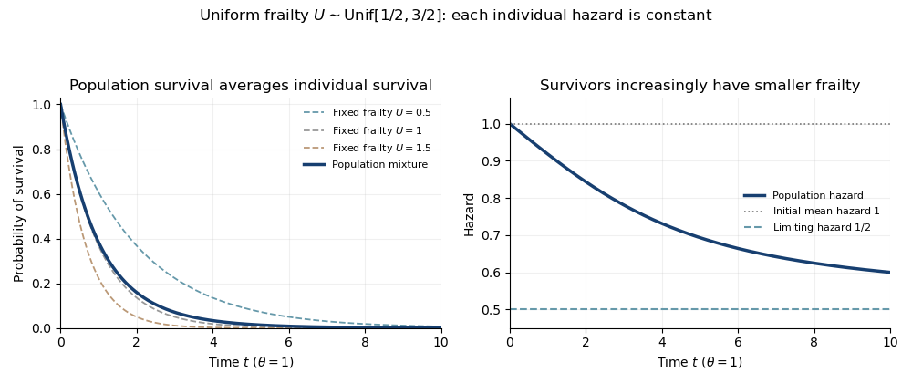
Uniform frailty survival mixture and declining population hazard despite constant individual hazards
. Details. 
The figure takes . The population survivor curve averages conditional exponential curves, while its hazard falls from the initial mean to the minimum individual hazard.
Articles by others on the same topic
There are currently no matching articles.