Past exam of the mathematics course of the University of Cambridge / 2007 / iii / Paper 68 (Stellar and Planetary Magnetic Fields)

Use the method of multiple scales, treating $t$ and $\tau =t/ϵ$ as independent variables, so differentiation becomes ${\partial }_t+{ϵ}^{-1}{\partial }_{\tau }$. Write $L={\partial }_x^2-{\ell }^2$ and average over a fast period $2\pi /|\omega |$, with $\omega \ne 0$. The fluctuations can depend slowly on $x,t$ as well as periodically on $\tau$. The ${ϵ}^{-1}$ balance in the poloidal magnetic field potential equation isIntegrating and imposing zero fast average determinesAt order one, the toroidal magnetic field equation is ${\partial }_t\overline{B}+{\partial }_{\tau }\tilde{B}=\Omega {\partial }_x(\overline{A}+\tilde{A})+L\overline{B}$. Its average and fluctuating parts give, respectively,Consequently the zero-average fluctuation isThe order-one averaged poloidal magnetic field potential equation retains the correlation between the fluctuating alpha effect and the fluctuating toroidal magnetic field. Although alpha has zero average, its product with the magnetic fluctuation does not:Thus the rapidly fluctuating alpha effect produces the leading averaged equationsA higher-order zero-average correction to $A$ accommodates the remaining fast order-one terms; it does not alter this leading averaged balance. These equations describe the small-$ϵ$ limit, rather than an exact finite-$ϵ$ identity.

For a Fourier mode, let $(\overline{A},\overline{B})=(a,b)e^{ikx+\sigma t}$ and put $d=k^2+{\ell }^2$. Then $(\sigma +d)a=-ikCb$ and $(\sigma +d)b=ik\Omega a$. Their determinant gives the dispersion relationHere $\Omega C={\Omega }^2{\alpha }_0^2/(2{\omega }^2)\ge 0$, so both growth rates are real. For a prescribed nonzero wavenumber, growth requires $\Omega C>(k^2+{\ell }^2{)}^2/k^2$. If real wavenumbers can be chosen freely, the largest growth rate occurs at $|k|=\sqrt{\Omega C}/2$ and is $\Omega C/4-{\ell }^2$. Hence growing averaged modes exist precisely whenA bounded or periodic spatial domain instead requires an admissible wavenumber satisfying the preceding mode-by-mode inequality.

The physical feedback differs from an ordinary Parker dynamo wave. A constant alpha effect couples $B$ directly into $A$, while the Omega effect differentiates $A$ once, producing the factor $ik\alpha \Omega$ responsible for an oscillatory phase. Here the fast alpha effect first creates a potential fluctuation in temporal quadrature; shear creates a magnetic fluctuation correlated with alpha. The averaged feedback is consequently proportional to $-{\partial }_x\overline{B}$. Combining its spatial derivative with the derivative in the Omega effect gives the real positive factor $\Omega C{k}^2$. In fact $({\partial }_t-L{)}^2\overline{B}=-\Omega C{\partial }_x^2\overline{B}$. The resulting growing fields have fixed spatial phase, so the leading averaged pattern grows without travelling. Fast within-period oscillations of the original fields remain present.

Here $\alpha$ is the thermal expansion coefficient and $\rho$ is the mass density. Let $K=|\mathbf{k}|$, $h^2=K^2-k_z^2$, $q=\mathbf{B}\cdot \mathbf{k}$, and $a^2=q^2/({\mu }_0\rho )$, the squared Alfvén frequency. We initially consider a nonzero frequency. The temperature and magnetic equations for a Fourier mode giveIn particular, the minus sign in the magnetic relation follows from $-i\omega \hat{\mathbf{b}}=iq\hat{\mathbf{u}}$. Substitution into the magnetohydrodynamic momentum equation, with $P=p/\rho$, givesFor incompressible flow, $\nabla \times (\hat{\mathbf{z}}\times \mathbf{u})=-{\partial }_z\mathbf{u}$. Taking the vertical component of the curl eliminates pressure and gives, with $\hat{\zeta }=(i\mathbf{k}\times \hat{\mathbf{u}}{)}_z$,Taking another curl and its vertical component uses $\nabla \times \nabla \times \mathbf{u}=-{\nabla }^2\mathbf{u}$ and $(\nabla \times \nabla \times (\theta \hat{\mathbf{z}}){)}_z=h^2\hat{\theta }$. Thusor, after eliminating temperature,The two equations for vertical velocity and vertical vorticity have a nontrivial solution only when their determinant vanishes. This proves the stratified magneto-Coriolis wave dispersion relationNo division by $\Delta$ was necessary, so a possible $\Delta =0$ is retained. Division by $\omega$, however, was necessary. Stationary disturbances must be checked directly in the original equations: for example, with $q\ne 0$, $\mathbf{u}=0$ and an appropriate solenoidal magnetic perturbation can balance temperature-induced buoyancy and pressure. Such static balances are separate from the nonzero-frequency wave branches.

Keep the background magnetic field, thermal gradient and wavevector fixed as $|\Omega |\to \infty$. In particular, $k_z/K$ is nonzero and of order one. Put $H=g\alpha \beta$ and $X={\omega }^2$. Multiplying the nonzero-frequency dispersion relation by ${\omega }^2$ givesthat is,The sum and product of its two roots areFor large rotation, the sum is of order ${\Omega }^2$ while the product is independent of $\Omega$. The quadratic therefore has one large root and one small root. More explicitly,The fast frequencies are consequentlywhich are inertial waves at leading order. For nonzero $a$ away from the zero-frequency boundary, the rapid-rotation slow magneto-Coriolis branch hasIts frequency is of order $|\Omega {|}^{-1}$, much smaller than the fast inertial wave frequency. Coriolis force balances most of the magnetic and buoyant forces in this slow motion, with inertia supplying only a small correction.

For $a^2>0$, the slow wave has real nonzero frequency whenStable thermal stratification has $H<0$ and automatically satisfies this condition. With adverse stratification, $H>0$, sufficiently strong magnetic tension along the wavevector is needed. If the inequality is reversed, $X_s<0$ and the slow branch has imaginary frequencies, including an exponentially growing mode. Equality gives a stationary limit, rather than a nonzero oscillation. If $\mathbf{B}\cdot \mathbf{k}=0$, the proposed slow wave degenerates into zero-frequency disturbances: there is no magnetic restoring coupling. The remaining nonzero branch has ${\omega }^2=(4{\Omega }^2{k}_z^2-H{h}^2)/K^2$. These qualifications also explain why zero roots introduced by clearing denominators must not be interpreted as ordinary propagating waves.

Take the coupling parameters to be real. The dipole and quadrupole parity in a mean-field dynamo subspaces are invariant: substitution of $A_2=A_1$, $B_2=-B_1$ makes the second-hemisphere equations equal to the first-hemisphere equations with these same signs. Substitution of $A_2=-A_1$, $B_2=B_1$ likewise preserves the other parity. In either subspace put $A=A_1$, $B=B_1$. The reduced equations and characteristic equations areA marginal normal mode has $\lambda =i\omega$. Equating real and imaginary parts givesConsequently the marginal surfaces areTo identify which side actually grows, write $z=ab$ in $(\lambda +1{)}^2=z$. The largest real part of the two eigenvalues is $-1+\sqrt{(|z|+\mathrm{Re}z)/2}$. It is negative exactly when $\mathrm{Re}z+[\mathrm{Im}z{]}^2/4<1$: squaring $|z|<2-\mathrm{Re}z$ proves this, and the latter condition ensures the right-hand side is positive. Thus dipole modes decay for $F_d<1$ and quadrupole modes decay for $F_q<1$, with growth for the corresponding reversed inequality.

For explicit coupled-hemisphere dynamo parity thresholds, suppose $\Omega \ne 0$ and defineThe dipole stability interval is $\delta -L<{\alpha }_0<\delta +L$, and the quadrupole stability interval is $-\delta -L<{\alpha }_0<-\delta +L$. A comparison of first onset from ${\alpha }_0=0$ assumes both are initially stable, namelyIncrease $|{\alpha }_0|$ along a specified sign $s=\mathrm{sgn}{\alpha }_0$. The first thresholds for the two parities areTherefore the quadrupole reaches onset first if $s({\Omega }^2{ϵ}_1+2{ϵ}_2)>0$; the dipole reaches onset first if it is negative; the thresholds coincide if it vanishes. For positive ${\alpha }_0$ and positive coupling parameters this selects the quadrupole, provided the initial stability condition holds. Reversing the sign of ${\alpha }_0$ exchanges the preference. If both signs are freely allowed, each parity attains the same minimum threshold $|\Omega |(L-|\delta |)$ on opposite sign rays; a unique preference cannot be inferred from the absolute product alone. If the initial stability condition fails, the zero-alpha state is already unstable or marginal and there is no first onset from a stable origin. When $\Omega =0$, the formulas for $F_d,F_q$ still apply, but $|{\alpha }_0\Omega |$ is identically zero and is not a useful onset parameter.

For an alpha-quenching rotating wave, write the four complex fields as constant amplitudes times $e^{i\omega t}$, with $\omega$ real. The squared toroidal amplitudes are then constant, so the algebraic alpha quenching coefficients are constant on the orbit. Assume $\Omega \ne 0$. With ${ϵ}_2=0$, the toroidal equations determineSubstitution in the potential equations gives the amplitude eigenvalue problemThe matrix is real symmetric, hence Hermitian, and every one of its eigenvalues is real. For a nonzero amplitude vector this forces $1-{\omega }^2=0$. Thus every nonzero rotating wave of this form hasSet $a={\alpha }_0-2\omega /\Omega$. In the dipole subspace $B_2=-B_1$ and $A_2=A_1$; in the quadrupole subspace $B_2=B_1$ and $A_2=-A_1$. The amplitude equations giveThese are nonzero waves exactly when the respective squared amplitude is positive. A common constant phase of $B_1,B_2$ is arbitrary, and $|A_j{|}^2=2|B_j{|}^2/{\Omega }^2$. In particular, choosing $\omega =\mathrm{sgn}\Omega$, both parities exist once ${\alpha }_0>2/|\Omega |+|{ϵ}_1|$. The other frequency sign is also algebraically possible whenever its positivity conditions hold; existence alone says nothing about stability of that branch.

There is a genuine sign qualification in the polynomial alpha quenching law. It subtracts $p|B{|}^2$ independently of the sign of ${\alpha }_0$. Thus a sufficiently large positive ${\alpha }_0$ gives the intended waves, but a sufficiently large negative ${\alpha }_0$ makes every displayed squared amplitude negative for both frequency signs. For example, with $\Omega =1$, ${ϵ}_1=0$, ${\alpha }_0=-M$ and $M>2$, neither $(-M-2)/p$ nor $(-M+2)/p$ is nonnegative. Large $|{\alpha }_0\Omega |$ alone is insufficient as printed; positive alpha, or the exact amplitude-positivity conditions above, is required. A sign-preserving quenching prescription would be a different model.

For the unequal-hemisphere dynamo rotating wave, first take ${ϵ}_1\ne 0$. The real symmetric matrix above has distinct eigenvalues because its off-diagonal entry is nonzero. Its eigenvector is real up to a common complex phase, so choose $B_1=b_1$, $B_2=b_2$ real. The amplitude equations reduce toMultiplying the first equation by $b_2$, the second by $b_1$, and subtracting givesFor unequal magnitudes, therefore, $b_1{b}_2=-{ϵ}_1/p$. Neither amplitude can vanish. Multiplying the first amplitude equation by $b_1$ then shows $ap{b}_1^2-p^2{b}_1^4-{ϵ}_1^2=0$. Equivalently,The two distinct positive roots exist precisely when $a>2|{ϵ}_1|$. This constructs the desired solutions explicitly:Choose $b_1$ to be either square root of the first value, and set $b_2=-{ϵ}_1/(p{b}_1)$; substituting verifies both amplitude equations. Interchanging the two roots gives the hemisphere-exchanged companion. The hinted choice $\omega =1$ therefore requires ${\alpha }_0-2/\Omega >2|{ϵ}_1|$. At equality the magnitudes coincide, so it is not an asymmetric solution. For ${ϵ}_1>0$ the amplitudes have opposite signs and meet the dipole branch at equality; for ${ϵ}_1<0$ they have the same sign and meet the quadrupole branch.

If ${ϵ}_1=0$, the hemispheres decouple. An asymmetric rotating wave instead has one hemisphere inactive and the other with $|B{|}^2=a/p>0$. If both hemispheres are active their magnitudes must be equal, although their relative phase is arbitrary. If $\Omega =0$, the toroidal equations simply give ${\dot{B}}_j=-B_j$, so no nonzero common-frequency rotating wave exists.

The unequal-amplitude solutions describe a periodically reversing dynamo concentrated more strongly in one hemisphere, with $|A_1|\ne |A_2|$ following from $|A_j|=\sqrt{2}|B_j|/|\Omega |$. Both $B_d=(B_1-B_2)/2$ and $B_q=(B_1+B_2)/2$ are nonzero, so the field combines the two dipole and quadrupole parity in a mean-field dynamo classes rather than belonging to either one. Equatorial reflection exchanges the two companion solutions. The model can therefore break hemispheric symmetry without asymmetric input parameters. This construction proves existence; nonlinear stability would require an additional perturbation calculation.

Magnetoconvection is the competition between thermally driven convection and the force and transport of a conducting fluid's magnetic field. An imposed magnetic field resists motions that bend its field lines through magnetic tension, while magnetic diffusion permits slippage. The competition changes the onset threshold, preferred spatial scale, temporal behaviour and finite-amplitude organization. The geometry matters: a disturbance nearly invariant along a horizontal imposed magnetic field can avoid much of its tension, whereas an impermeable layer with a vertical imposed magnetic field cannot generally avoid bending it.

A useful quantitative example is a nonrotating Boussinesq layer of depth $d$, heated from below with temperature drop $\Delta T>0$ and threaded by a vertical magnetic field $B_0\hat{\mathbf{z}}$. Let $\nu$, $\kappa$, $\eta$ denote kinematic viscosity, thermal diffusivity and magnetic diffusivity. In thermal-diffusion units define the Rayleigh number, Prandtl number, magnetic-to-thermal diffusivity ratio and Chandrasekhar number byUse stress-free impermeable boundaries, fixed temperature perturbation zero, and magnetic boundary conditions keeping the field vertical. More explicitly, the normal modes below satisfy $w={\partial }_z^{2}w=\theta =b_x=b_y={\partial }_z{b}_z=0$ at $z=0,1$. For a horizontal wavenumber $a>0$, take $w,\theta \propto \sin \pi z$, $b_z\propto \cos \pi z$, and put $s=a^2+{\pi }^2$. The linear temperature and resistive induction equation give $(\lambda +s)\theta =w$ and $(\lambda +\zeta s)b_z={\partial }_{z}w$. Applying the solenoidal projection to the magnetohydrodynamic momentum equation removes pressure; the magnetic coupling is $Q\zeta {\partial }_z\mathbf{b}$, and the vertical projected buoyancy has coefficient $R{a}^2/s$. Substituting the temperature and magnetic responses gives the vertical-field magnetoconvection dispersion relationThese stated boundary conditions make the single vertical mode exact in this model; other boundaries change numerical thresholds.

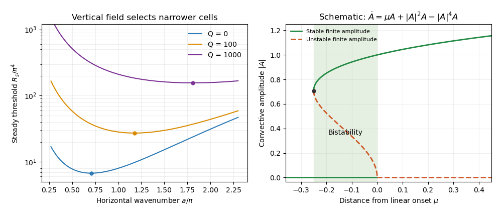
For steady marginal convection, set $\lambda =0$. The threshold curve isThe imposed magnetic field adds a positive penalty. Differentiating with respect to $x=a^2$ shows that the minimizing wavenumber obeysAt $Q=0$ this gives $a_c=\pi /\sqrt{2}$ and $R_c=27{\pi }^4/4$. With increasing $Q$, the root moves to larger $x$ because the left-hand side is strictly increasing for $x\ge {\pi }^2/2$. The strong-field wavenumber selection in magnetoconvection limit isThus a strong vertical imposed field raises the steady threshold and selects narrower convection cells. At small horizontal wavenumber the incompressibility constraint makes a given vertical motion require large horizontal displacement and magnetic bending. Increasing horizontal wavenumber reduces this magnetic penalty, but increases viscous and thermal diffusion. Their balance selects the narrow cells. This statement is specific to the vertical-field geometry: wavenumber selection in oblique-field magnetoconvection can instead favour nearly field-invariant motions.

Oscillatory marginality in vertical-field magnetoconvection occurs because magnetic and temperature perturbations need not relax at the same rate. To exhibit the phase balance, substitute $\lambda =i\omega$ with $\omega \ne 0$ and write the neutral condition asThe imaginary part must vanish because $R$ is real. Dividing that imaginary part by $\omega s$ givessoA nonzero oscillation consequently requires $0<\zeta <1$ and a sufficiently strong imposed magnetic field. In this regime thermal diffusion can erase the temperature anomaly faster than magnetic diffusion relaxes bent field lines. The magnetic restoring force can outlast the buoyant anomaly, reverse the motion, and maintain the phase lag needed for oscillatory instability. The real part gives the oscillatory neutral curveOnly its portions with ${\omega }^2>0$ are physical. The first onset is the lower of the minimized steady and admissible oscillatory thresholds; the existence of an oscillatory neutral solution at a given wavenumber alone does not establish that it is first. For example, at fixed $P>0$ and $0<\zeta <1$, both minimizing wavenumbers grow like $Q^{1/6}$ for large $Q$, while $R_s\sim {\pi }^{2}Q$ and $R_o\sim D{\pi }^{2}Q$ with $D=\zeta (P+\zeta )/(1+P)<1$. At those oscillatory minima, the positive order-$Q$ contribution to ${\omega }^2$ dominates its order-$Q^{2/3}$ negative contribution, so the oscillatory branch is genuinely admissible and becomes the lower threshold. An overstability therefore precedes steady onset in this limit. More generally nonlinear convection can oscillate even when linear onset is steady; the linear calculation is not a classification of every time-dependent state.

The nonlinear regime introduces a different feedback. The magnetic Reynolds number $\mathrm{Rm}=Ud/\eta$ measures induction relative to diffusion for a finite convective velocity $U$. At large but finite $\mathrm{Rm}$, persistent convection rolls can redistribute magnetic flux. In a two-dimensional incompressible roll, a flux function $\mathcal{A}$ obeysCirculation repeatedly stretches the flux pattern, building gradients on which even small magnetic diffusivity acts efficiently. Over the flux-rearrangement time this permits flux expulsion: the interior of a vigorous roll becomes weakly magnetized, while magnetic flux is concentrated near its edges. The weak-field interior then suffers less magnetic inhibition and can support broader, stronger convection than the linear narrow-cell prediction for the original uniform magnetic field. Exact zero resistivity would preserve material flux and cannot by itself justify the relaxed flux-expelled state.

The weak interior field also follows from a steady leading-order balance for a coherent two-dimensional roll. Let $\psi$ be its streamfunction and suppose its interior streamlines are nested closed curves with $\nabla \psi \ne 0$. In the small-diffusivity interior, $\mathbf{u}\cdot \nabla {\mathcal{A}}_0=0$ implies ${\mathcal{A}}_0=F(\psi )$. Integrate the full steady flux equation over the region enclosed by one streamline. Because $\mathbf{u}\cdot \mathbf{n}=0$ there, the advection integral vanishes; the divergence theorem then gives $\oint {\partial }_n\mathcal{A}ds=0$. In a regular interior expansion this requires $F^{\prime }(\psi )\oint {\partial }_n\psi ds=0$. The normal derivative of $\psi$ has one nonzero sign around a regular nested streamline, so $F^{\prime }(\psi )=0$. Hence the leading interior flux function is constant, and its spatial gradient, which gives the two-dimensional magnetic field, vanishes. The mismatch with external flux is accommodated by magnetic boundary layers. This argument assumes the coherent steady roll and a regular interior; it does not prove that every turbulent flow expels flux.

The mean imposed vertical magnetic flux is conserved for horizontally periodic boundaries. In a schematic two-region picture, let a fraction $f$ have weak field $B_c$ in vigorous convection and the remainder have field $B_q$. ThenThe intensified field outside the active cells inhibits surrounding convection. This gives magnetic flux separation: vigorous weak-field patches coexist with strong-field regions whose motion is small or occurs on a finer scale. The redistribution is a consequence of nonlinear induction and back reaction, rather than disappearance of the net imposed flux.

This feedback can permit subcritical magnetoconvection. Infinitesimal perturbations decay below the conductive state's linear threshold because they encounter the full imposed field. A finite-amplitude roll can nevertheless persist by first expelling enough flux to reduce its own magnetic restraint. A sufficient finite disturbance can then switch between the stable conductive state and a convective state, producing hysteresis. A schematic amplitude equation makes the distinction between local linear stability and finite-amplitude persistence explicit:Here $\mu$ measures distance from linear onset; this is an illustrative normal form, not a claim that these coefficients have been derived for every magnetic layer. Writing $r=|A{|}^2$, the nonzero equilibria satisfyThey appear at a saddle-node bifurcation at $\mu =-c^2/(4d)$. For $-c^2/(4d)<\mu <0$, the zero state is stable, the lower radial-amplitude branch is unstable, and the upper branch is stable because its radial derivative has sign $c-2d{r}_{+}<0$. Thus finite-amplitude convection can coexist with a linearly stable conductive state below the onset threshold. Large $\mathrm{Rm}$ facilitates the flux-expulsion mechanism but is not a universal sufficient condition: geometry, the imposed magnetic field, the capacity to form coherent recirculating cells, and magnetic back reaction all matter. The broad nonlinear cells in weak-field regions can coexist with much narrower cells in magnetically dominated regions, linking the nonlinear flux distribution back to scale selection.