Past exam of the mathematics course of the University of Cambridge / 2010 / iii / Paper 12 (Probabilistic Combinatorics)

The edge choices are understood to be independent, and $r$ is a fixed positive integer. We prove the hypergraph extension property and then show directly that it determines a unique countable hypergraph isomorphism type.

For a finite $S\subseteq \mathbb{N}$, prescribe a family $\mathcal{A}\subseteq \left(\genfrac{}{}{0ex}{}{S}{r-1}\right)$. We want a new vertex $v$ such thatFor any $v\notin S$, the probability of precisely this pattern in the countable random uniform hypergraph isTwo different candidate vertices use disjoint hyperedge decisions: all the other vertices in each tested edge lie in $S$. The successes are therefore independent random variables with the same positive probability $q$. The probability that the first $N$ candidates all fail is $(1-q{)}^N\to 0$. The same argument after discarding any finite initial set of candidates shows that infinitely many witnesses exist almost surely.

There are only countably many finite subsets of $\mathbb{N}$, and finitely many prescriptions for each. A countable union of null events is null. Consequently the random uniform hypergraph satisfies every such extension prescription simultaneously almost surely.

Now let $H$ and $K$ be two countably infinite $r$-uniform hypergraphs with the hypergraph extension property. Enumerate their vertex sets and construct increasing finite partial hypergraph isomorphisms by the back-and-forth method. At a forward step, take the least unused vertex $u$ of $H$. Its incident hyperedges with each $(r-1)$-subset of the current domain specify a pattern on the matched vertices of $K$. The hypergraph extension property supplies an unused vertex $v$ of $K$ with exactly this pattern. Adding $u\mapsto v$ preserves and reflects every hyperedge in the enlarged domain. At the next step, take the least unused vertex of $K$ and perform the identical construction with $H$ and $K$ interchanged.

The union of the finite maps is defined on every vertex and has every vertex in its range. It is a bijection, and each finite $r$-set appears at some finite stage, so all hyperedges and nonedges are preserved. Thus it is a hypergraph isomorphism. Existence of at least one structure with the property follows from the probability-one construction already proved; fix one representative and call it $G_{\mathrm{univ}}^{(r)}$. ThereforeThe hypergraph isomorphism type does not depend on $p$. In the case $r=2$ it is the Rado graph. For $r=1$, the argument says that the infinitely many selected and unselected singleton vertices determine the same one-uniform structure for every $p\in (0,1)$.

The printed assertion is false when maximal means largest in the natural-number labelling. Both the original PDF and the TeX have this wording. The specified operation gives the complete graph, not the Rado graph.

Fix any two distinct vertices $u,v\in \mathbb{N}$, and choose $M\ge \max \{u,v\}$. Apply the hypergraph extension property of $G_{\mathrm{univ}}^{(3)}$ to $S=\{1,\dots ,M\}$, prescribing that the pair $\{u,v\}$ extend to a hyperedge; prescribe all other pairs in $S$ arbitrarily. The resulting witness $w\notin S$ has $w>M$, so $\{u,v,w\}$ is a hyperedge whose largest vertex is $w$. Deleting that vertex produces the edge $\{u,v\}$ in $G_0$.

Since $u,v$ were arbitrary,The Rado graph has nonedges: its hypergraph extension property supplies a new vertex nonadjacent to any specified existing vertex. Therefore $K_{\mathbb{N}}$ and $G_{\mathrm{univ}}^{(2)}$ cannot be isomorphic graphs. This argument holds for every representative of the universal three-uniform structure labelled by $\mathbb{N}$, so changing its labelling does not repair the assertion. Equivalently, in an independently sampled representative each pair has infinitely many larger vertices that complete it to a triple, almost surely.

A valid related construction is to fix a vertex $a$ and take its link hypergraph: make $\{u,v\}$ an edge exactly when $\{a,u,v\}$ is a hyperedge, on the remaining vertex set. This is indeed the Rado graph. To prove it, take any disjoint finite sets $U,W$ of vertices other than $a$, put $S=\{a\}\cup U\cup W$, and prescribe triples through the pairs $\{a,u\}$ for $u\in U$ and no triples through $\{a,w\}$ for $w\in W$. Complete all other pair prescriptions arbitrarily. The hypergraph extension property produces a new vertex adjacent in the link to all of $U$ and none of $W$. Uniqueness from part (i), for $r=2$, now proves the claimed hypergraph isomorphism for this corrected operation.

Use the uniform probability measure on the symmetric group $S_n$ and the unnormalized Hamming distanceLet $f:S_n\to \mathbb{R}$ have Lipschitz constant $K>0$ for this distance. We will prove the one-sided concentration inequalitiesConsequently $\mathbb{P}(|f-\mathbb{E}f|\ge t)\le 2e^{-t^2/(2n{K}^2)}$ for $t>0$. A zero Lipschitz constant makes $f$ constant, so that case is immediate.

Let $\sigma$ be a uniform permutation, reveal $\sigma (1),\dots ,\sigma (k)$ successively, and define the Doob exposure martingaleFix the first $k-1$ images. For an available value $a$, let $h(a)$ be the conditional mean when $\sigma (k)=a$. Given two available values $a,b$, left-composition with the transposition exchanging $a,b$ is a bijection from completions with next image $a$ to completions with next image $b$. It fixes the previously exposed images and changes exactly two coordinates of each complete permutation. Since conditional completions are uniform, averaging the Lipschitz condition over this pairing gives $|h(a)-h(b)|\le 2K$.

Thus, conditionally on the first $k-1$ images, $M_k-M_{k-1}$ has mean zero and takes values in an interval of length at most $2K$. We need the range-length version of the Hoeffding lemma: if a real random variable $Z$ has mean zero and lies in an interval of length $\ell$, thenHere is a proof. For $\psi (\lambda )=\log \mathbb{E}{e}^{\lambda Z}$, differentiation gives ${\psi }^{\prime \prime }(\lambda )={\mathrm{Var}}_{\lambda }(Z)$ under the exponentially tilted probability distribution. Any distribution on an interval of length $\ell$ has variance at most ${\ell }^2/4$, because its squared distance from the interval midpoint is at most ${\ell }^2/4$. Since $\psi (0)={\psi }^{\prime }(0)=0$, integrating this second-derivative bound gives the lemma for both signs of $\lambda$. The same argument holds for every conditional distribution.

Apply it conditionally to each martingale difference and use the tower property of conditional expectation repeatedly:The exponential Markov bound now gives, for $\lambda >0$,Choose $\lambda =t/(n{K}^2)$ to obtain the upper tail in the box, and apply the argument to $-f$ for the lower tail. This proves concentration of Lipschitz functions on the symmetric group. Using only the bound $|M_k-M_{k-1}|\le 2K$ in the absolute-increment Azuma-Hoeffding inequality would lose a factor four in the exponent; the conditional range length is what yields the constant needed in part (ii).

Put $d=d_H(A,B)=\min \{d_H(\alpha ,\beta ):\alpha \in A,\beta \in B\}$, and define $f(\sigma )=d_H(\sigma ,A)$. The triangle inequality shows that $f$ is Lipschitz continuous with Lipschitz constant one. It vanishes on $A$, and $f\ge d$ on $B$. Let $\mu =\mathbb{E}f$ for a uniform permutation.

If $\mu \ge d/2$, apply the lower-tail bound proved in part (i):If $\mu <d/2$, apply its upper-tail bound:For $d=0$ the desired inequality is simply $\min \{|A|,|B|\}\le n!$. Hence in all casesThis uses only the precise one-sided concentration inequality from part (i) and the Hamming distance triangle inequality. The normalization of the distance matters: it counts mismatching coordinates, rather than dividing their number by $n$.

Take the sampled points to be independent with the uniform distribution on $T=\{(x,y):0\le y\le x\le 1\}$. Its area is $1/2$, so its probability density is two. With probability one there are no coincidences, equal relevant coordinates or collinear triples. We give an exact first moment method argument; no tangent construction is needed.

First count the probability that $k$ labelled points, together with the endpoints, form a convex chain. In their order along the lower boundary, write their coordinates as $(x_i,y_i)$, $1\le i\le k$, and put $(x_0,y_0)=(0,0)$, $(x_{k+1},y_{k+1})=(1,1)$. They necessarily satisfyIndeed the lower boundary of the convex polygon is the graph of a convex piecewise linear function. Its segment slopes strictly increase; the first is positive because the first point lies above the $x$ axis, making all later slopes positive too.

Set $u_i=x_i-x_{i-1}$ and $v_i=y_i-y_{i-1}$ for $1\le i\le k+1$. Both spacing vectors lie in the open probability simplex, with ${\sum }_i{u}_i={\sum }_i{v}_i=1$. The coordinate-monotone region has volume $1/(k!{)}^2$. The change to the first $k$ spacings in each vector has Jacobian one, and each simplex has uniform volume measure. Simultaneous permutation of all $k+1$ pairs $(u_i,v_i)$ preserves this product volume measure. Except on a null set of ties, the ratios $v_i/u_i$ therefore have all $(k+1)!$ possible orders with equal volume.

Strict increase of these ratios is exactly the convex chain condition. It also puts the intermediate points below the diagonal: the weighted mean of all slopes is ${\sum }_i{u}_i(v_i/u_i)=1$, and each proper initial weighted mean is strictly smaller than one, so $y_j<x_j$ for $j\le k$. Thus it suffices to impose the slope order on the whole coordinate-monotone region; no additional triangle restriction is needed.

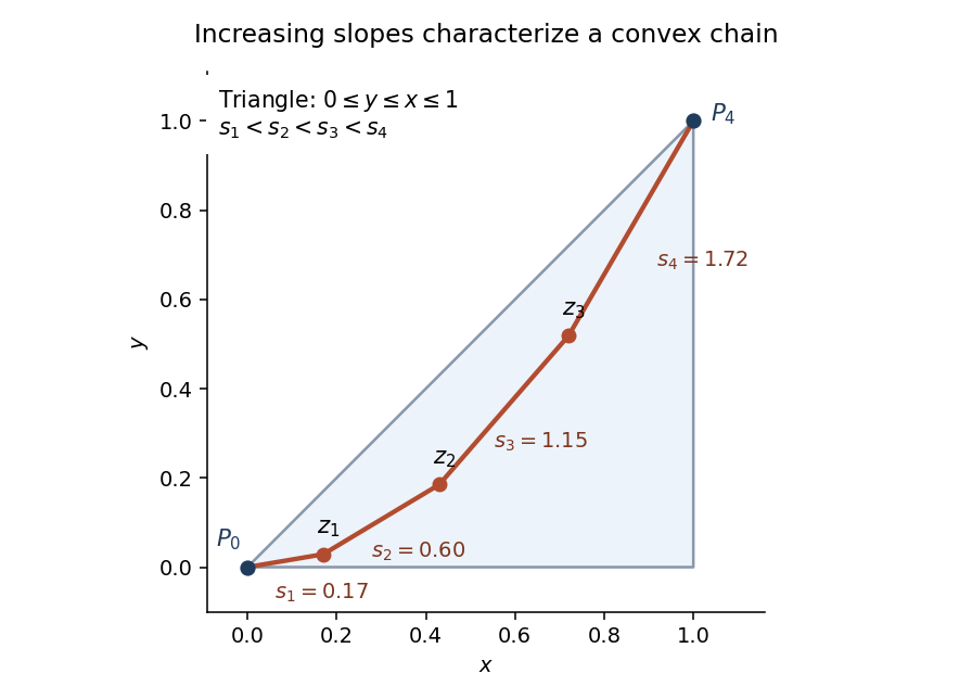
The volume for one specified label order is consequently $1/((k!{)}^2(k+1)!)$. There are $k!$ disjoint orders of the labels, and the joint uniform-triangle density is $2^k$. Hence the convex-chain probability in a triangle isFor example $p_1=1$ and $p_2=1/3$.

Let $C_k$ count the $k$-element subsets of the $n$ sampled points that are convex chains. By linearity of expectation, $\mathbb{E}{C}_k=\left(\genfrac{}{}{0ex}{}{n}{k}\right)p_k$. If $L_n\ge k$, an optimal chain contains a $k$-vertex subchain, since removing vertices from a convex polygon preserves convex position of the remaining vertices. Therefore, by the first moment method,We used $\left(\genfrac{}{}{0ex}{}{n}{k}\right)\le n^k/k!$, $(k+1)!\ge k!$, and $k!\ge (k/e{)}^k$, the last following from ${\sum }_{j=1}^k\log j\ge {\int }_1^k\log xdx$.

Take $k=\lceil 4e{n}^{1/3}\rceil$. If $k\le n$, the last bound is at most $32^{-k}<1/2$; if $k>n$, the event is empty. Every integer median $m_n$ must then satisfy $m_n<k$, and thereforeThe hint's curve $y=x^2$ is a parabola, not a hyperbola. The exact counting argument above proves the upper bound directly. The same chain probability is recorded in Ambrus and Bárány's analysis of longest convex chains.

We use the directed set version of the Talagrand convex distance:Here a coordinate is an entire sampled point, so $x_i\ne y_i$ means the two planar points differ. This is the distance from the upper event $A$ to the lower event $B$; its order is relevant because the convex distance need not be symmetric.

Fix $x\in A$ and choose exactly $a$ indices $I$ whose points form a convex chain with the endpoints. Such a choice exists even if $L_n(x)>a$, by taking a subchain. It is a certificate of the certifiable function $L_n$. For any $y\in B$, let $J=\{i\in I:x_i\ne y_i\}$. The $a-|J|$ unchanged selected points remain a convex chain in configuration $y$, soChoose the nonnegative weights ${\alpha }_i=a^{-1/2}$ for $i\in I$ and zero otherwise. They have squared sum one, and for every $y\in B$,Taking the infimum over $y$, then the supremum over weights, and finally the infimum over $x\in A$ provesThis proof also works for $b=0$ if zero-length chains are admitted, and gives the usual infinite separation when one of the events is empty. For the uniform sampling model, $L_n\ge 1$ almost surely when $n\ge 1$.

The precise external concentration result we use is Talagrand's convex distance inequality: for a finite product of independent standard probability spaces, a measurable event $B$ of positive probability, and $u\ge 0$,Our coordinates are the independent uniformly sampled points of the triangle, so the hypothesis holds. Part (ii) therefore gives, for integers $a>b\ge 0$,Indeed every configuration in the first event has at least the distance from part (ii) to the second event. If one event is empty, the displayed product bound is automatic. This is the only use of the product-space theorem; the geometric separation was proved directly in part (ii). A precise source for that theorem is Section 4.1 of Talagrand's original product-space concentration paper.

Choose an integer median $m=m_n$, so $\mathbb{P}(L_n\le m)\ge 1/2$ and $\mathbb{P}(L_n\ge m)\ge 1/2$. First set $a=m+t$, $b=m$ in the product bound, and then set $a=m$, $b=m-t$. For positive integers $t$ this yields the convex-chain median concentration estimatesThe lower event is empty if $m-t<1$ in our sampling model; the upper event is empty if $m+t>n$. Thus the stated bounds remain valid for all positive integers $t$. Also $m\ge 1$ for $n\ge 1$.

By part (i), $m\le C{n}^{1/3}$ with $C=4e$. Let $h_n=\omega (n)n^{1/6}/2$, take $t_n=\lfloor h_n\rfloor +1$, and use the deterministic interval $I_n=[m-h_n,m+h_n]$. Its length is exactly $\omega (n)n^{1/6}$. As $L_n$ and $m$ are integers, falling outside this interval implies one of the two tail events with $t=t_n$. ThereforeFor positive $m,t$,Since $t_n\ge h_n$ and $m\le C{n}^{1/3}$, this exponent is at leastConsequentlyThus $L_n$ lies with high probability in the required interval. This proof works for every $\omega (n)\to \infty$, including growth faster than $n^{1/6}$; no extra restriction on $\omega$ is needed. The scale comes from the square root of the $O(n^{1/3})$ certificate size at the median.

Let $i(G)$ be the number of independent sets of the biregular graph $G$. Choose one such set $I$ uniformly and write $X_v=1_{v\in I}$. All information entropies below use logarithms to base two, soWe will prove $\boxed{i(G)\le (2^r+2^s-1{)}^{m/s}}$.

We state and justify the entropy facts used. For a finite-valued random variable $Y$, $H(Y)=-{\sum }_y{p}_y{\log }_2{p}_y$ with $0{\log }_{2}0=0$. Its conditional entropy is the mean of this quantity over the conditioning variable. Factoring the joint probabilities proves the chain rule for information entropy, $H(Y,Z)=H(Y)+H(Z\mid Y)$. Conditioning reduces entropy: $H(Y\mid Z,T)\le H(Y\mid Z)$. To see this, condition on $Z$ and use concavity of $-x{\log }_{2}x$ to compare the mixture of the conditional distributions given $T$ with their mean entropy.

The precise Shearer inequality needed here is: if subsets $S_j$ of the indices of a finite random vector $Y$ cover every index at least $d$ times, then $dH(Y)\le {\sum }_{j}H(Y_{S_j})$. To prove it, order the indices. The chain rule for information entropy expandsThe inequality is conditioning reduces entropy. Summing over $j$ counts each nonnegative conditional term at least $d$ times and proves the assertion.

For every $w\in W$, its vertex neighbourhood $N(w)\subseteq U$ has $s$ vertices. Every $u\in U$ lies in exactly $r$ of these neighbourhoods. Hence Shearer inequality givesLet $q_w=\mathbb{P}(X_{N(w)}=0)$, the probability that no neighbour of $w$ is selected. Conditional on a particular selected subset of $U$, a vertex $w$ with a selected neighbour is forbidden, and all other vertices of $W$ are available. Because there are no edges within $W$, every subset of the available vertices is a valid completion. Uniform choice of $I$ makes these completions equally likely. The available coordinates are therefore independent fair binary choices, each of entropy one, and the forbidden coordinates are zero. Averaging their number givesBy the chain rule for information entropy,It remains to bound each bracket. Let $Y=X_{N(w)}$, a binary vector of length $s$, with distribution $(p_y)$ on $\{0,1{\}}^s$, and put $Z=2^r+2^s-1$. Assign weight $w_0=2^r$ to the all-zero vector and weight $w_y=1$ to every nonzero vector. ThenThe first inequality is Jensen's inequality for the concave logarithm; the weights sum to $2^r+(2^s-1)$. This explicitly handles zero probabilities and does not assume the neighbourhood indicators are independent.

There are $n$ right vertices, so combining the bounds and using $rm=sn$ givesExponentiating proves the required independent-set bound for biregular graphs. The proof uses both degree constraints: $r$ supplies the neighbourhood-cover multiplicity and the conditional-completion weight, while $s$ determines the number of neighbourhood patterns.

Write $q=m/s$, an integer under the stated divisibility assumption. The degree relation gives $n=rm/s=qr$. Take the disjoint union of graphs of $q$ copies of the complete bipartite graph $K_{s,r}$, placing its $s$-vertex part in $U$ and its $r$-vertex part in $W$. The total part sizes are then $qs=m$ and $qr=n$. Each left vertex has vertex degree $r$, and each right vertex has vertex degree $s$, so the graph has exactly the required biregular graph parameters.

An independent set in one component can be any subset of its left part or any subset of its right part. It cannot contain a vertex from both parts, because all cross-pairs are edges. The two families share only the empty set, so the component has $2^s+2^r-1$ independent sets. Choices in different connected components of a graph are independent combinatorial choices, and their counts multiply. HenceThis attains equality in part (i). It also explains the entropy weight $2^r$ there: the empty selected left neighbourhood permits all $2^r$ subsets of the opposite part.