Past exam of the mathematics course of the University of Cambridge / 2010 / iii / Paper 35 (Mathematics of Operational Research)

Use the optimization Lagrangian with the sensitivity sign conventionFor equality constraints the Lagrange multipliers have unrestricted signs. The Lagrangian sufficiency theorem says that if $h(x^{\ast })=b$ and, for some ${\lambda }^{\ast }$, $x^{\ast }$ globally minimizes $L_b(\cdot ,{\lambda }^{\ast })$ over $X$, then $x^{\ast }$ globally minimizes $f$ subject to the constraint. Indeed every feasible $x$ satisfiesThis proves the theorem without a convexity or differentiability assumption. Merely finding a stationary point of the optimization Lagrangian would not establish its required global minimum.

Let $\varphi (u)=\inf \{f(x):x\in X,h(x)=u\}$, with value $+\infty$ when the feasible set is empty, and suppose $\varphi (b)$ is finite. The problem has the Strong Lagrangian property if a finite multiplier $\lambda$ satisfiesThis includes attainment of the dual bound by a multiplier. It does not by itself assert attainment of the primal infimum. For every multiplier, restricting the infimum to feasible $x$ gives ${\inf }_X{L}_b(x,\lambda )\le \varphi (b)$, the relevant weak duality. A non-vertical supporting hyperplane of a value function is a planewith $\varphi (u)\ge \varphi (b)+{\lambda }^T(u-b)$ for every $u$. Its vertical coefficient is nonzero and has been normalized to one; the epigraph lies above it. The two directions of the equivalence are proved in parts (a) and (b).

For the sampling allocation put $A={\sum }_i\sqrt{a_i{v}_i}$. Finite variance requires every $x_i>0$; interpret the objective at a zero coordinate as $+\infty$. An optimum uses all the budget, because scaling every positive $x_i$ up would otherwise reduce the objective while remaining feasible. The Cauchy-Schwarz inequality gives the global boundEquality requires $v_i/x_i$ to be proportional to $a_i{x}_i$. The budget then determines the unique allocation:This is the optimal cost-constrained stratified sampling allocation.

For an inequality ${\sum }_i{a}_i{x}_i\le b$, our sign convention uses $\lambda \le 0$, so $L_b=f-\lambda ({\sum }_i{a}_i{x}_i-b)$ is a lower bound on $f$ at feasible points. Its coordinate stationary equations are $-v_i/x_i^2-\lambda a_i=0$, and the displayed allocation givesThe function $v_i/x_i+(-{\lambda }^{\ast })a_i{x}_i$ has a strict global minimum at $x_i^{\ast }$: its second derivative is $2v_i/x_i^3>0$ and its value diverges at both endpoints of $(0,\infty )$. Thus the multiplier also supplies the Lagrangian sufficiency theorem certificate, with the tight inequality giving complementary slackness.

Finally, for $b+\delta b>0$,Hence the first-order change in minimal variance is $\boxed{{\lambda }^{\ast }\delta b}$. Increased resources decrease the variance. With the alternative convention $L=f+\mu ({\sum }_i{a}_i{x}_i-b)$, the multiplier is $\mu =-{\lambda }^{\ast }>0$ and the sensitivity is $-\mu \delta b$.

Suppose the non-vertical supporting hyperplane of a value function has slope $\lambda$. Every $x\in X$ then satisfiesso $L_b(x,\lambda )\ge \varphi (b)$. Taking the infimum gives ${\inf }_X{L}_b\ge \varphi (b)$. Conversely, feasible points approaching the infimum of $f$ have $L_b=f$, so ${\inf }_X{L}_b\le \varphi (b)$ even if no primal minimizer exists. Thereforewhich is the Strong Lagrangian property.

If the Strong Lagrangian property holds with multiplier $\lambda$, its infimum identity implies, for every $x\in X$,For any feasible right-hand side $u$, take the infimum over $h(x)=u$ to obtainThe inequality also holds at infeasible $u$, where $\varphi (u)=+\infty$, and it is equality at $u=b$. Thus $r=\varphi (b)+{\lambda }^T(u-b)$ is the required non-vertical supporting hyperplane of a value function. This proves the converse and completes the equivalence. Neither implication requires that $X$ be a convex set.

Introduce nonnegative slack variables $s_1,s_2$ and let $z$ denote profit. We display each simplex tableau as coefficients of its row equation, with the coefficient of $z$ in the objective equation implicitly one. Thus a negative coefficient in the last row permits an improving entering variable. The initial simplex tableau isUse the simplex method with $x_2$ entering. The simplex ratio test gives ratios $6/2=3$ and $6/1=6$, so $s_1$ leaves. Divide its row by two and eliminate the other $x_2$ entries:Next $x_1$ enters. The positive-column ratios are $3/(1/2)=6$ and $3/(3/2)=2$, so $s_2$ leaves. After this pivot and a row reordering,The last row is $z=14-(5/3)s_1-(2/3)s_2$, so every nonnegative feasible solution has $z\le 14$. Setting the nonbasic variables to zero givesThe equality certificate also shows uniqueness, since both nonbasic objective coefficients are strictly unfavorable.

Add the slack variable $s_3$ for the forgotten constraint. In the optimal simplex tableau from part (a), $x_1+x_2=4-(s_1+s_2)/3$. Hence the new row in canonical form isAppending it givesThe objective row remains dual feasible, but $s_3=-1$ makes the basic solution infeasible. Apply the dual simplex algorithm: $s_3$ leaves, and the eligible columns are $s_1,s_2$, whose negative coefficients can repair this row. The dual ratio test comparesThus $s_2$ enters. Pivoting on $-4/3$ and eliminating its column givesAll basic values are nonnegative and the objective equation is $z=27/2-s_1-s_3/2$. ThereforeBoth binding constraints have zero slack, and the final objective row proves global optimality. The two nonbasic penalties are strictly positive, so this optimum is unique.

The old slack variable $s_3$ is exactly the amount now sold, so rename its column $y$. No further slack is added: the PDF specifies an equality. The feasible equations are otherwise unchanged. If $z_0$ is the old profit, the new profit is $z=z_0+y$. Substituting this into the old objective equation givesThis is the simplex objective update for a priced slack variable. The altered simplex tableau isThe coefficient $-1/2$ makes $y$ an improving entering variable. Its only positive constraint-row coefficient is $1/2$ in the $x_1$ row, whose ratio is $(3/2)/(1/2)=3$. Thus $x_1$ leaves. The simplex method pivot givesThe objective equation $z=15-x_1$ proves optimality. One optimal basic solution isThe zero reduced cost of $s_1$ permits alternative optima. In fact all optimal solutions areThese satisfy both remaining inequalities, and the equality then makes their profit exactly fifteen.

For a finite directed flow network with source $s$, sink $t$ and nonnegative finite flow network edge capacities $c_e$, the max-flow min-cut theorem statesHere feasible arc flows satisfy $0\le f_e\le c_e$ and flow conservation at every vertex except $s,t$. Their strength of a flow is the net outflow at $s$. A cut of a flow network has cut capacity equal to the sum of capacities on arcs directed from $S$ to $S^c$.

For any feasible flow and any such cut of a flow network, summing flow conservation over $S$ cancels internal arcs and givesThus every flow value is bounded by every cut capacity.

A maximum flow exists: the feasible arc-flow vectors form a nonempty closed subset of the finite-dimensional compact box ${\prod }_e[0,c_e]$, and flow value is continuous. Choose one, $f^{\ast }$. Its residual network has a forward arc of capacity $c_e-f_e^{\ast }$ and a reverse arc of capacity $f_e^{\ast }$ for each original arc. If a residual $s$–$t$ augmenting path existed, its smallest positive residual capacity would permit increasing forward flows and decreasing reverse flows along the path. This preserves all capacity bounds and internal flow conservation while strictly increasing $|f^{\ast }|$, a contradiction.

Let $S$ be the vertices reachable from $s$ through positive residual arcs. Then $t\notin S$. Every original arc leaving $S$ is saturated, since otherwise its endpoint would also be reachable. Every original arc entering $S$ carries zero flow, since a positive flow would create a residual reverse arc leaving $S$. ThereforeTogether with the universal upper bound, this proves both optimality claims and the theorem. This existence argument works for real capacities; it does not assume that arbitrary choices in the Ford-Fulkerson algorithm terminate. For integer capacities, positive augmentations are integral and increase the flow value by at least one, so the algorithm does terminate.

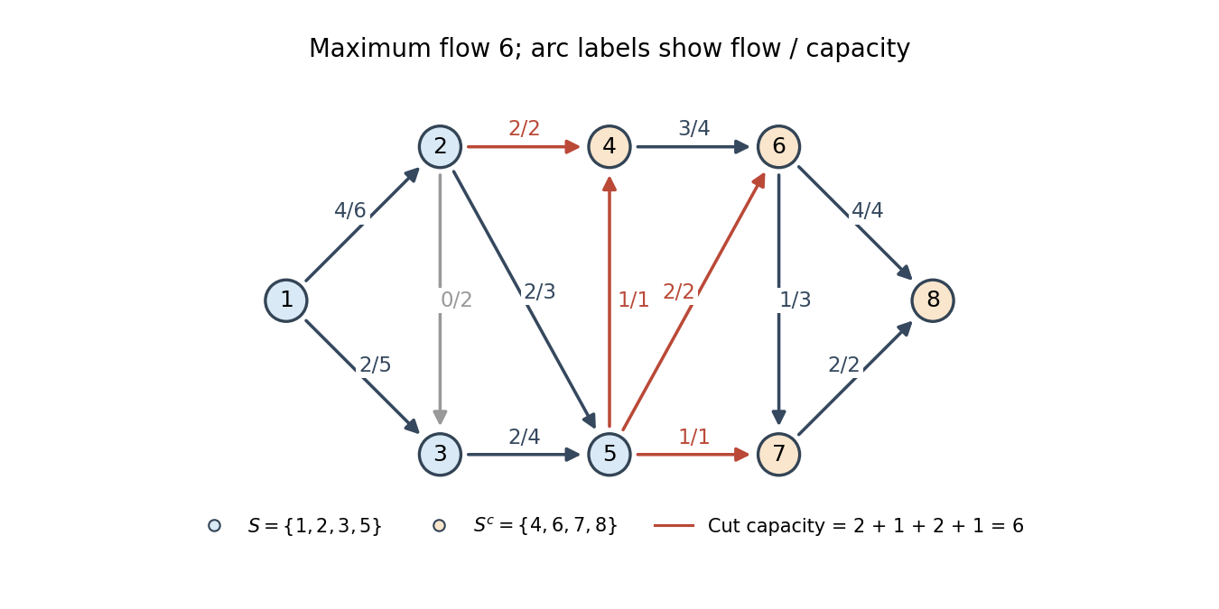
Start with zero flow and apply the Ford-Fulkerson algorithm. The following augmenting paths and bottlenecks use the capacities in the original PDF diagram:For example, the second path is limited by the remaining capacity two on $6\to 8$ and by capacity two on $5\to 6$. After the third augmentation, $7\to 8$ has residual capacity one; the fourth path supplies it through $5\to 4\to 6\to 7$. Every displayed increment is the smallest residual capacity of its path.

The resulting arc flows areHere $uv$ denotes $u\to v$. These satisfy every capacity bound and flow conservation. The final residual network has source-reachable set $S=\{1,2,3,5\}$. Its outgoing arcs are $2\to 4$, $5\to 4$, $5\to 6$ and $5\to 7$, with capacities $2,1,2,1$, all saturated. ConsequentlyThis is a minimum cut, and the equal flow and cut values certify optimality by the max-flow min-cut theorem. The cut immediately before node eight also has capacity six, so the minimum cut is not unique.

Use the transportation simplex algorithm, with transportation dual potentials $u_i,v_j$ and reduced costs $r_{ij}=c_{ij}-u_i-v_j$. On a basic cell choose $u_i+v_j=c_{ij}$. The initial shipment matrix, read from the circled entries in the PDF, isIts six positive cells form a transportation spanning tree. Setting $u_1=0$ givesEnter cell $(1,1)$, whose reduced cost is $-6$. The cycle pivot has signsThe maximum feasible increment is $\theta =\min (5,4)=4$, so cell $(4,1)$ leaves the basis. The result isFor the new transportation spanning tree,Enter cell $(2,3)$ with reduced cost $-4$. Its cycle pivot isNow $\theta =\min (5,1)=1$, and cell $(1,3)$ leaves. We obtainIts row sums are $(12,5,7,12)$ and its column sums $(9,14,13)$, as required. The final transportation dual potentials areAll reduced costs are nonnegative, proving optimality. More explicitly, for any feasible shipment matrix $X$,Our shipments use only zero-reduced-cost cells and attain this lower bound. This supplies an independent weak duality certificate for the transportation optimum.

Let $t_k\in \{0,1\}$ encode the truth value of $X_k$. For a Boolean literal $\ell$, write $L_{\ell }(t)=t_k$ if $\ell =X_k$ and $L_{\ell }(t)=1-t_k$ if $\ell ={\overline{X}}_k$. A clause is true precisely when the sum of its literal values is at least one. Thus the integer programming formulation of satisfiability is the feasibility problemwith objective zero. Every feasible binary vector gives a satisfying assignment of the Boolean satisfiability problem, and conversely. An empty clause gives $0\ge 1$ and hence infeasibility.

For maximum satisfiability, introduce binary variables $q_i$ marking clauses selected as satisfied and solveA false clause forces $q_i=0$, while a true clause permits $q_i=1$. At an optimum every permitted $q_i$ is one, since increasing it improves the objective without affecting another constraint. Therefore the objective is exactly the maximum number of simultaneously true clauses. Repeated literals cause no difficulty, and a clause containing both signs of a variable is always true.

For the literal-frequency greedy approximation for MAX-SAT, keep only clauses not already satisfied and remove literals made false. Count occurrence in clauses, rather than multiplicity within a clause. At a step let $a$ be the number of current clauses containing the chosen literal $z$, and $b$ the number containing its opposite $\overline{z}$. Since $z$ has maximum clause frequency among all remaining literals, $b\le a$.

Setting $z$ true permanently satisfies exactly the $a$ clauses containing it. Some other clauses may become empty and are then permanently lost. Every newly empty clause previously contained $\overline{z}$, so their number $d$ satisfiesA clause containing both signs is satisfied and cannot be one of the lost clauses. Repeat this accounting at every step. Satisfied clauses are removed, so no success is counted twice; each lost nonempty original clause becomes empty at exactly one step. If $G$ is the total number satisfied and $D$ the number of initially nonempty clauses lost, summing the inequalities gives $D\le G$. Every initially nonempty clause eventually falls into one of these two classes. Writing their number as $N_{+}$, we getEven an optimal assignment can satisfy at most $N_{+}$ clauses. ConsequentlyThus Greedy is a $1/2$-approximation in the convention stated in the question. The proof also covers initial empty clauses by excluding them from $N_{+}$; they are unsatisfiable for every algorithm.

A coalitional game with transferable utility has a finite player set $N$ and a characteristic function of a coalitional game $v:2^N\to \mathbb{R}$, normalized by $v(\varnothing )=0$. The value $v(S)$ is the total payoff the coalition $S$ can secure and redistribute among its members.

An imputation is an efficient, individually rational payoff vector:The core of a cooperative game consists of imputations satisfying every coalition constraint:A coalition assigned less than its characteristic value can leave and make every member better off, by sharing the positive surplus. Conversely a coalition with no such surplus cannot improve every member's payoff simultaneously. This explains the stability represented by the core of a cooperative game.

It is useful to prove the general core of the miners game calculation when $r$ miners carry one unit: $v(S)=\lfloor |S|/r\rfloor$, with $r\ge 2$. Individual rationality gives $x_i\ge 0$, and efficiency gives ${\sum }_i{x}_i=q:=\lfloor n/r\rfloor$.

If $n<r$, the grand coalition value is zero and the only core allocation is zero. If $n\ge r$, every $r$-person coalition must receive at least one. Sum these inequalities over all $\left(\genfrac{}{}{0ex}{}{n}{r}\right)$ such coalitions. Each player appears $\left(\genfrac{}{}{0ex}{}{n-1}{r-1}\right)$ times, soIf $r$ does not divide $n$, then $rq<n$, a contradiction. Thus the core of a cooperative game is empty in these cases.

If $n=r$, every proper coalition has value zero. The core is exactly the simplex of nonnegative allocations with total one. If $n$ is a multiple of $r$ with $n\ge 2r$, the averaged inequality is equality. Since each $r$-person coalition sum is at least one, every such sum equals one. For any two players $i,j$, choose $r-1$ other players and compare the two resulting $r$-person coalition sums. They imply $x_i=x_j$. Hence $x_i=1/r$ for all players. This vector belongs to the core because $|S|/r\ge \lfloor |S|/r\rfloor$ for every coalition.

For two miners per lump, therefore,In particular the even case has a small-group exception at $n=2$.

For three miners per lump, the same proof givesThus divisibility controls the existence of a stable allocation once enough miners are present, while exactly one possible lump leaves freedom to divide its value.

Let $L$ be the set of left-shoe owners and $R$ the right-shoe owners. This is the glove game with pair price ten, so its characteristic function of a coalitional game isAll singleton values are zero. Write ${\ell }_i\ge 0$ for left-owner payoffs and $r_j\ge 0$ for right-owner payoffs. Efficiency gives total $10\min (a,b)$, and each mixed pair imposes ${\ell }_i+r_j\ge 10$.

Suppose $a<b$. Removing any right owner leaves at least $a$ right shoes, so the complement coalition still has value $10a$. Its core inequality and efficiency imply $r_j\le 0$. Thus every right owner receives zero. The pair constraints then force ${\ell }_i\ge 10$, and their total is $10a$, so every left owner receives ten. Conversely this allocation gives each coalition $10|S\cap L|$, at least its value, so it is in the core. The argument is symmetric when $a>b$.

When $a=b=k$, sum all $k^2$ mixed-pair inequalities. Their total left side is $k$ times the grand-coalition payoff, namely $10k^2$. Hence every inequality is equality: ${\ell }_i+r_j=10$ for every pair. Fixing one right owner shows all left payoffs are the same $\theta$, and fixing one left owner shows all right payoffs are $10-\theta$. Individual rationality gives $0\le \theta \le 10$. Such allocations are sufficient: for a coalition with $u$ left owners and $v$ right owners,as is seen by subtracting the right side and factoring either $\theta (u-v)$ or $(10-\theta )(v-u)$.

The core of a glove game is thereforePayoffs are in pounds. The parameter in the balanced case is common to all owners of a given shoe type.

The payoff $e(x,z)$ is the expected fitness of an individual using strategy $x$ against a population using strategy $z$. The resident $x^{\ast }$ is initially common; the mutant $y$ is introduced at small frequency $ϵ$. Convexity of the strategy set makes their population mixture admissible. If residents have higher expected fitness in every sufficiently small invasion by a fixed mutant, selection works against that mutant: this is an evolutionarily stable strategy. The allowed upper bound on $ϵ$ may depend on $y$.

For expected payoffs of mixed strategies, $e(x,z)$ is affine in the population strategy $z$; in a finite matrix game it is $x^{T}Az$. This property is the basis of the two-condition criterion for evolutionary stability. For fixed $y\ne x^{\ast }$, putAffineness gives the exact invasion differenceIf this is positive for all sufficiently small $ϵ>0$, taking $ϵ\downarrow 0$ gives $A_y\ge 0$. If $A_y=0$, the difference is $ϵB_y$, so necessarily $B_y>0$. Conversely, if $A_y>0$, it remains positive for sufficiently small $ϵ$: for example take $ϵ<A_y/(A_y+|B_y|)$. If $A_y=0$ and $B_y>0$, it is positive for every $ϵ>0$. Applying this argument separately to every $y$ provesThus an evolutionarily stable strategy is a symmetric Nash equilibrium with an additional condition against tied mutants. For a general nonlinear interaction function on a convex set, affineness would be an additional necessary hypothesis for this particular equivalence; here it follows from the mixed-strategy expected-payoff interpretation. For example, on $X=[0,1]$ take $e(x,z)=xz(x/2-z)$ and resident $x^{\ast }=0$. For every $y>0$, $A_y=0$ and $B_y=y^3/2>0$, but at population $ϵy$ the mutant earns $ϵy^3(1/2-ϵ)>0$ while the resident earns zero. Thus the two conditions alone would not suffice for an arbitrary nonlinear $e$; the expected-payoff assumption is used explicitly.

For the Hawk-Dove game, let $p$ be an individual's Hawk probability and $q$ the population's Hawk probability. The given matrix yieldsWe use this formula in each case. In the usual interpretation, resource value $V$ and damage cost $D$ are positive. The parts below also specify the boundary or negative-value alternatives because positivity is not written explicitly in the PDF.

Take pure Hawk, $p^{\ast }=1$. For every mutant $p<1$, the payoff difference against an all-Hawk population isThe strict first condition of the two-condition criterion for evolutionary stability holds for every mutant. ThereforeThis conclusion holds even without the usual positivity assumption on the two parameters.

For $V=D>0$, choose pure Hawk. Every mutant $p<1$ ties it against a resident Hawk population, so the second condition must be checked. The Hawk-Dove game formula givesConsequentlyThe actual invasion advantage is $ϵV(1-p{)}^2/2>0$, despite the tie at invasion frequency zero.

If the equal parameters are negative, pure Dove is instead an evolutionarily stable strategy: for a mutant $p>0$, $e(0,0)-e(p,0)=-pV/2>0$. If $V=D=0$, every payoff is zero and no resident has a strict advantage over any mutant. Thus the full equal-parameter answer is Hawk for $V=D>0$, Dove for $V=D<0$, and no ESS for $V=D=0$.

In the usual positive-parameter case $0<V<D$, set $p^{\ast }=V/D\in (0,1)$. Every mutant ties the resident against the resident population, because $V-D{p}^{\ast }=0$. Against a mutant population, however,The second condition of the two-condition criterion for evolutionary stability holds, soIndeed its advantage at invasion frequency $ϵ$ is exactly $ϵD(p^{\ast }-p{)}^2/2$. The interior frequency balances the two pure-strategy payoffs in the Hawk-Dove game.

For completeness, if $V<D$ but $V<0$, pure Dove is an evolutionarily stable strategy by the strict inequality $e(0,0)-e(p,0)=-pV/2>0$ for every mutant $p>0$. If $V=0<D$, that difference is zero, but $e(0,p)-e(p,p)=D{p}^2/2>0$, so Dove again satisfies the second condition. Thus for the remaining allowed values $\boxed{x^{\ast }=(0,1)\text{ when }V\le 0<D\text{ or }V<D\le 0}$; equivalently, Dove works whenever $V<D$ and $V\le 0$.