For independent binomial distributions in the two trial arms, the estimate of the log risk ratio isThe delta method gives ; replacing by the sample proportion gives , where is the event count. Adding the independent arm contributions therefore givesThe standard error is . Using the stipulated normal quantile two, the approximate confidence interval isThe point estimate of the risk ratio is , corresponding to approximately 79% lower mortality risk in the transfusion arm. Exponentiating the endpoints gives an approximate 95% confidence interval for the risk ratio of . It includes one, so the trial is compatible with no difference as well as substantial benefit or some harm. The point estimate favours transfusion, but the data are too imprecise to establish a difference at the 5% level. These are large-sample approximations, especially rough with only one event in an arm. A frequentist confidence interval describes repeated-sampling coverage, not a 95% posterior probability for this fixed parameter.
Let be each trial's estimated log risk ratio, with estimated sampling variance . A fixed-effect meta-analysis models the independent estimates as , with one common true log risk ratio . Differentiating the Gaussian log-likelihood, or minimizing , gives inverse-variance weights andThe variance follows directly by adding independent variances of the weighted estimates: .
Using the printed rounded estimates and standard errors, , soThe pooled risk ratio is about . An interval using the same quantile two is on the log scale, so it includes no effect. Recomputing all trial estimates from the event counts would change the last digits because the printed log estimates and errors are rounded.
The key assumptions are independent trials, a common true treatment effect on this chosen log scale, approximately unbiased and approximately normal trial estimates, and suitable sampling-variance estimates. The common-effect assumption is stronger than merely studying the same named treatment: systematic population, treatment or design differences may produce genuine heterogeneity. For an unbiased interpretation of the pooled evidence, inclusion of studies must also not depend selectively on their results. Treating the plug-in variances as fixed is the usual approximation in the displayed variance formula.
Publication bias occurs when the availability or publication of a study depends on its results, for example their direction or statistical significance. The published studies then need not represent all studies meeting the review's eligibility criteria. This is different from unbiased studies simply having large sampling errors.
If mortality reductions favouring transfusion are more likely to be published than null or unfavourable findings, the observed log risk ratios will tend to be too negative and the pooled risk ratio too small. The apparent benefit will then be exaggerated. An ordinary meta-analysis interval ignores uncertainty about the missing evidence and may have poor coverage even if its sampling-variance calculation is correct for the studies included. The direction of bias depends on which results are preferentially made available; publication bias does not invariably favour a particular treatment.
A funnel plot places each estimated log risk ratio horizontally and its standard error vertically, with the most precise studies at the top. Under a common-effect model without selective availability, less precise estimates should spread approximately symmetrically around the underlying effect. The plotted dashed limits are the pooled estimate plus or minus twice the standard error; they illustrate the expected sampling spread, not a test of publication bias by themselves.
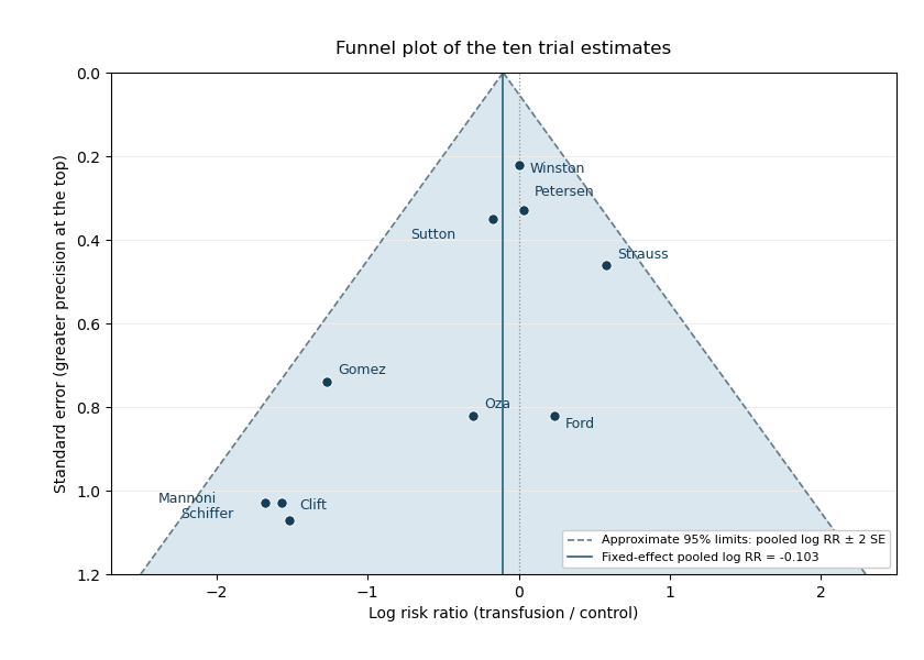
Funnel plot of the ten transfusion trial estimates, with inverse-variance pooled effect and approximate sampling limits
. The least precise estimates are mostly far to the left, whereas the most precise estimates are close to zero. The reported regression slope means that increasing the standard error by one unit is associated with a decrease of about in the estimated log risk ratio. Its 95% confidence interval excludes zero, and gives evidence against a zero slope under that regression model. This is evidence of a small-study effect: less precise trials report stronger apparent benefit.
There is evidence consistent with publication bias, but asymmetry does not identify its cause. Selective availability of favourable small studies is a plausible explanation. Genuine differences in patient populations, trial quality, interventions or effect modification could also generate the pattern, and there are only ten trials. The given outcome-on-error regression should be interpreted as specified; it is not automatically the original standardized-effect-on-precision form of an Egger test. The plot and slope justify investigating missing studies and sensitivity to selection, rather than concluding that publication bias has been proved.
One method is trim and fill. Estimate the direction and extent of funnel asymmetry, temporarily trim the extreme studies on the overrepresented side to estimate a centre, and fill in mirror-image studies on the underrepresented side. Recompute the pooled effect using the observed and imputed studies. This estimates what the summary might be under a symmetry-based missing-study model. It can move an exaggerated effect towards the null, but genuine heterogeneity can violate its symmetry assumptions.
A second method is a selection model for publication bias. Specify how the probability of a result being available depends on quantities such as its value, direction or precision, and combine that mechanism with a model for the underlying study effects. If a study estimate has density and availability probability , its observed density is proportional to , with a normalizing factor accounting for unobserved results. Fit the model, or vary the selection probabilities over plausible scenarios, to obtain selection-adjusted effects. Such models make assumptions about evidence that is missing, so their results are particularly useful as sensitivity analyses. Neither method removes publication bias without assumptions about the missing studies.
Label batches before consulting the random-number table, so their labels are independent of the test results. A uniformly random permutation of , restricted to a smaller label set, induces a uniformly random ordering of that set. This provides a simple rejection-and-restriction scheme:
- For A, label each day's six batches . Use a fresh permutation, discard labels , and test the first remaining batch. Repeat independently on each working day. Each daily batch has inclusion probability , and five batches are tested per week.
- For B, label the fifteen weekly morning batches . Discard label 16 from a fresh permutation and choose the first three remaining labels. Use an independent permutation for the afternoon stratum. Every three-element subset within a stratum is equally likely, and each batch has inclusion probability . Six batches are tested per week.
- For C, label the weekdays . Keep the first label in this range from a fresh permutation and test all six batches on that day. Repeat independently each week. Every day, and hence every batch, has inclusion probability ; six batches are tested per week.
With independent random digits instead, rejection sampling gives the same uniform choices: for A keep only digits ; for C keep only . For B, use uniform two-digit numbers, retain labels , and reject repeats within a three-batch sample. Taking residues modulo six or fifteen from a table whose range is not divisible by that number would give unequal probabilities. These are respectively day-stratified simple random sampling, morning/afternoon stratified sampling, and a one-day design using cluster sampling. The printed word “rest” for A is interpreted as “test”, consistently with the surveillance task. If it instead meant leaving one batch untested, choose that omitted batch uniformly and test the other five; this alternative would test 25 batches per week, with inclusion probability , and has a different testing budget.
Under the one-test-per-day interpretation, A spreads surveillance across all five days and is operationally straightforward, but uses only five tests per week and does not guarantee morning/afternoon representation. Within each day its uniform choice avoids systematically selecting a particular batch. B uses six tests, guarantees representation of both production periods, and spreads the selected batches over the week's production, though some weekdays can receive no test. C also uses six tests and may minimize the cost of collecting samples, but concentrates them on one randomly selected day.
If batches produced on the same day share contamination risks, C's six observations are positively correlated and provide less information than six dispersed batches. A simple equal-cluster-size approximation has design effect , where is within-day intraclass correlation; its effective sample size is consequently smaller than six when . C can also miss intermittent problems occurring on other days.
I would prefer B for estimating and comparing batch contamination rates, assuming positive within-day correlation and no overriding collection-cost advantage for C. It combines slightly more testing than A with explicit production-period coverage and avoids C's concentration on a single day. A is a reasonable alternative when regular daily surveillance is the priority. All three are legitimate probability samples with the stated inclusion probabilities; the preference concerns precision and coverage, not a claim that C is intrinsically biased. Their relative efficiency is not universal without a model for production variability and costs.
A numerical power calculation needs a significance level, desired power, sidedness and allocation; these are not specified in this part. For a concrete planning illustration, assume independent batches, equal samples per supplier, a two-sided 5% test with 80% power, and true rates and . The observed 2% from B and C is being used as a planning value for B, not as proof that B's population rate is exactly known. There is also a numerical inconsistency in the stated frame: at six batches per working day, B and C together produce only 120 batches in two weeks, and their proposed schemes would test 24. The asserted 3,000 sampled batches cannot literally come from that frame. The calculation treats as a stipulated planning estimate; its collection would require a larger frame or longer period.
For two independent sample proportions, the approximate null variance of their difference is and its variance at the alternative is , with . Separating the null critical value from the alternative mean by the required power quantile gives the sample size for comparing two proportions:With , and , this gives , so the normal-approximation calculation rounds to 1,141 batches per supplier, or approximately 1,150 for a practical planning target. This is per supplier, not the combined total. A different power or a one-sided test changes the answer. Positive clustering of sampled batches requires a cluster-aware calculation or inflation, so the independent-batch calculation should not simply be applied to C's one-day clusters.
For equal independent samples, take , and in the two-proportion formula, with two-sided and power . It givesThus the usual normal planning estimate isThe combined approximate design therefore checks about eight blocks, with about eight positive batches from B and twenty-four from C at the rounded design.
Those expected counts are low enough for test discreteness to matter. If a genuinely exact two-sided Fisher exact test is specified, the null allocation of the positive batches between two equal-size suppliers is hypergeometric, conditional on their total. Under the proposed alternative, its power is obtained by summing the independent binomial probabilities over the exact rejection region:An independent calculation of the exact power of Fisher's exact test gives about at and at . Consequently five whole 10,000-batch blocks per supplier suffice for at least 80% power with this conservative exact test. Four blocks are the intended normal-approximation answer, not an exact 80% guarantee irrespective of the chosen test. The distinction is a property of rare-event discreteness, not a change in the proposed effect size.
A group sequential design can stop early when the treatment is insufficiently promising, reducing expected recruitment, patient exposure and cost when the effect is poor. It also allows a planned decision before maximum enrollment.
A disadvantage is that the analysis is selected by the interim results: estimation and uncertainty must account for stopping, and power and operational planning depend on the stopping rule. The following parts quantify the resulting conditional estimation bias. If a design also allows repeated efficacy tests, its rejection boundaries must control overall Type I error. In the present futility-only design, stopping without rejection need not inflate the error rate of a single prespecified final test; it can make that test conservative. Earlier decisions are valuable, but the ordinary fixed-sample analysis is not automatically appropriate after selection.
At stage 1, the maximum-likelihood estimators of the two normal arm means are their sample means. Their difference estimates the treatment effect:Each arm has patients and variance , so independence across arms givesThe quantity is the Fisher information for the mean difference when the common variance is known. The PDF's preliminary expression uses for the variance denominator, although indexes arms and is not defined. The stage-specific sample size is ; the calculation uses this intended reading, consistent with the specified per-arm recruitment and the later weighted estimator. Fresh stage-2 patients are independent of stage-1 patients in the usual trial model; the cumulative stage means themselves are not independent across stages.
The Wald statistic has law . Write for continuation. By the normal cumulative distribution function,The final sample size per arm is , soIt lies between and , increasing with the treatment effect: a more promising treatment is more likely to reach full enrollment. Total expected recruitment over both arms is twice this expression. Equality at the futility boundary has probability zero under the normal model.
Conditioning on continuation selects the upper part of the stage-1 estimator's distribution, since . Thus for every finite threshold. The fresh stage-2 estimate is independent of and remains unbiased for . The pooled estimator retains a positive weight on the selected stage-1 data, givingConditional on full enrollment, the ordinary pooled MLE overestimates the treatment effect. This is conditional selection bias after futility continuation. Randomization of treatment assignments does not undo selection on the interim outcome.
For , set , and . Then . Symmetry of the normal density and distribution yieldsThe ratio is an Inverse Mills ratio. It is positive, and the pooled estimator's conditional bias is thereforeThis identity supplies both correction procedures below.
Both alternatives can be made explicit. For a conditional bias-corrected normal mean estimate, let be the observed pooled estimate and , with . Invert its conditional mean:This can be solved by bracketing or by Newton iteration . Since ,The variance of a standard normal conditional on exceeding is , strictly between zero and one. Positivity follows from nondegeneracy; the upper bound follows because the conditional mean exceeds the truncation threshold . Hence , so the equation has at most one root. As , ; as , the truncated stage-1 mean approaches its threshold and , so a root exists for every finite . Equivalently, differentiating the conditional likelihood divides the ordinary likelihood by and gives the same score equation. This conditional-likelihood correction is not exactly conditionally unbiased merely because it inverts a mean.
For an illustration, take , , and . The equation is . Since and , the corrected estimate lies between zero and ; numerical solution gives , below the selected ordinary estimate.
For the uniform minimum variance conditionally unbiased estimator, put , , and . The fresh estimate is conditionally unbiased because it is independent of continuation. LetBefore selection, conditional Gaussian calculations give . Conditional on as well, this normal variable is truncated below , soUsing , Rao-Blackwellization therefore givesIts conditional expectation is , and its conditional variance cannot exceed that of . To justify uniform minimum variance, the joint conditional density of is a base density on multiplied by . Thus is a complete sufficient statistic in the one-parameter conditional exponential family, whose natural parameter ranges over an open real interval. The Lehmann–Scheffé theorem proves the claim. The orthogonal pooled arm-average statistic is independent of the entire difference process and carries the nuisance common mean. Together with , it gives a complete sufficient statistic in the selected two-parameter normal family, with an open natural-parameter space. Thus allowing that nuisance statistic does not improve the conditional unbiased estimate of the difference. For the same illustration, , and give . It differs from the conditional-likelihood estimate because exact conditional unbiasedness is a different criterion.
Assume independent censoring: the censoring mechanism contributes no factor involving the lifetime rate . The exponential density and survival function are and . An observed event contributes the density; a right-censored lifetime contributes the probability of surviving its censoring time. Thus the likelihood for , up to censoring factors independent of it, isFor and , vanishes at , and proves the maximum:Censored individuals add follow-up time to the denominator but no event to the numerator. If and , the likelihood decreases for and has only a supremum as ; zero is an extended boundary estimate, not a positive-rate exponential MLE. The derivation is for independent individuals entering at time zero; delayed entry would require conditional survival contributions and exposure measured from entry.
Within month two, each individual contributes only the time spent at risk between times one and two. There are complete one-month contributions. The six event contributions are , and the censored contribution is . ConsequentlyThe month-specific likelihood factor in a piecewise-exponential survival model is , givingThe eight individuals no longer at risk at time one contribute no month-two exposure. Using either all 112 individuals or all 104 as full-month observations would give the wrong denominator.
The log-rank test compares survival experience through the allocation of events within the successive risk sets. Its null is equal hazard functions between the groups over follow-up, with independent individuals and noninformative censoring within groups. At each distinct event time , let be the numbers at risk immediately before that time, and let be event counts. Under the null, conditional on the total , the expected number of A events is .
The signed log-rank statistic is the observed-minus-expected scoreA positive score indicates relatively more A events than expected, hence a higher event hazard for A; B's score is its negative. Censoring times do not produce score terms, but remove people from all later risk sets.
At each event time the conditional null allocation is hypergeometric, as if the events were sampled without replacement from the risk set. Its variance gives the score-increment variance, with the finite-population correction for ties. Summing these conditional variances gives , since distinct-time martingale score increments have zero cross covariance under the null. For sufficiently many informative events, is approximately standard normal and approximately chi-squared with one degree of freedom. In the no-tie case, each variance contribution is . A time at which only one group remains at risk contributes no comparative information.
The numerical parts below report signed-score and variance contributions after day 160. They cannot be added as separate chi-squared statistics to the earlier follow-up: add the scores and variances first, and standardize once for the complete dataset. The log-rank test is particularly effective for proportional hazards alternatives; crossing hazards can produce cancelling score contributions.
At day 165 there are two A and two B individuals at risk. The event is in A, with expected A count , so its score contribution is and its variance contribution is . The remaining A individual is censored at 173 and leaves the risk set before either later event. The risk-set calculations are
ThusThe positive score indicates higher A event hazard in this late contribution. Although B has more observed events, its two events occur with no A individual at risk, so those times do not compare the groups. This is why raw event totals alone are insufficient for the log-rank test.
Keeping the event-free A individual under observation through day 193 leaves them in the risk set at both later B events. Now the calculations are
ThereforeThe negative score now indicates lower A event hazard, relative to B, in the contribution after day 160. The observed event counts have not changed. The change is in what events A was expected to contribute: its additional event-free exposure makes the two later B events informative comparisons, producing negative A score terms. No conclusion about the complete study's significance follows from this late contribution without the earlier scores and variances.
Use one row per consecutive at-risk episode, retaining a patient identifier for dependence and an episode number for event order. In calendar time, the intervals are ; status is one if the row ends in a headache and zero if it ends in censoring. Patient 001 contributes
The fifth episode is censored, not a fifth observed headache. All rows retain . This start-stop recurrent-event data layout corresponds to the counting-process intensity in survival analysiswhere indicates that the patient is currently observed and eligible for a headache. Fit the regression coefficient by Cox partial likelihood using the resulting risk sets, and estimate the baseline cumulative hazard nonparametrically, for example by the Breslow estimator. Patient rows are portions of one history, not new independent patients.
The second episode starts only after the first headache, at 24.8; its row is absent from every risk set before that time. More generally, episode starts at the observed end of episode . The left-open, right-closed interval convention assigns an event at a shared boundary only to the interval ending there. Thus the first event is counted once, and the second cannot be counted before the first. Preserving the episode entry times and patient history enforces the ordering; entering every recurrence as a new record starting at treatment time zero would not do so.
Set the availability indicator to zero during the three-day recovery interval after each headache. Keep each episode's endpoint, but delay its entry to the previous headache time plus three. The calendar-time rows become
The first interval still begins at zero because the patient was already headache-free for at least seven days before treatment. The recovery gaps supply no at-risk exposure and no partial-likelihood risk-set membership; they should not be retained as ordinary event-free at-risk time. If recovery extends past administrative closure, no subsequent eligible interval is created. This is a refractory period in recurrent-event analysis, represented by availability rather than by changing the event times.
For second and subsequent episodes, subtract the preceding headache time from both calendar endpoints. The new clock is the age since the start of that headache, not the age since recovery ended. Keeping the recovery restriction from part (c) therefore gives
For example, the second stop is , while its entry is . Thus subsequent rows begin at gap age three, not zero. The first row retains time since treatment started. Keep the patient and episode labels, and preferably the original calendar endpoints as auxiliary fields: gap ages in different episodes are not chronological treatment times. The value 7.1 for episode three being smaller than 8.3 for episode two does not reverse their occurrence order. This gap-time recurrent-event model forms risk sets on the episode-age scale while preserving each episode's historical eligibility.
Add a stratum indicator that is “First” for the first episode and “Later” for every subsequent episode, including the final censored episode:
A Stratified Cox model then uses distinct baseline hazards and , with a common treatment coefficient unless an interaction is explicitly desired. Form separate risk sets within the two strata and multiply their partial likelihoods. There is no need to force every later event number to have its own baseline when the stated aim is only first versus subsequent headaches. This is a first-event versus recurrent-event baseline stratification.
The episodes from one patient share treatment, biological susceptibility and prior history, so they are not independent observations. Treating every row as an unrelated subject can substantially understate uncertainty. Two approaches address this within-patient recurrent-event dependence:
- A patient-clustered sandwich covariance matrix retains a suitable working Cox mean/intensity model but groups score contributions by patient. If is the patient's score contribution and the observed information, its form is . Independent patients, rather than independent rows, determine the sampling units. This corrects uncertainty for within-patient dependence when the working estimating equation is appropriate; it does not repair an incorrect mean model.
- A shared frailty model introduces a common latent positive multiplier for all of patient 's episode hazards, often with a specified gamma or lognormal distribution. Given frailty and the relevant history, the event mechanism is modeled through that patient's intensity. Estimate treatment and frailty parameters by integrating or profiling the latent effect. This models persistent heterogeneity directly, but relies on the frailty assumptions and generally gives a conditional treatment-effect interpretation.
A patient-level bootstrap is another way to retain dependence: resample complete histories, not individual episode rows. It is not necessary to assume that robust marginal/working and frailty-conditional effect estimates target exactly the same parameter.
Begin by defining the scientific target: prediction for a new patient, or estimation of adjusted covariate effects. Check event definitions, follow-up origins, right-censoring codes and any delayed entry. The analysis assumes independent patients and censoring that is noninformative conditional on modeled covariates. For fixed explanatory variables , the Cox proportional-hazards model iswith an unrestricted baseline hazard and coefficients constant over time. Report as the conditional hazard ratio for a one-unit change in the coded variable, not as a risk ratio or automatically a causal effect.
For untied event times, fit the coefficients by maximizing the Cox partial likelihoodThe baseline cancels within each event risk set. Use an appropriate tied-event method, such as an Efron approximation or an exact method for a genuinely discrete event scale; the Breslow approximation for tied event times is another explicit approximation. Numerical score/information methods fit the model, and inverse information gives conventional covariance estimates for independent subjects. Report coefficient estimates, hazard ratios, uncertainty and the coding that makes their interpretation meaningful. After fitting, the Breslow estimator gives , from which provides predicted survival.
Adequacy is broader than significance of coefficients. Inspect influential observations, deviance residuals and data errors. Cox–Snell residuals should have approximately unit-exponential survival under a well-fitting model, retaining the original censoring indicators; a cumulative-hazard plot of these residuals should be near the 45-degree line. This is an overall diagnostic, not a substitute for the functional-form and proportionality checks below. For prediction, assess held-out discrimination and survival prediction calibration at prespecified time horizons with methods accounting for censoring. A high concordance index alone does not establish good calibration or correct hazard structure.
Use bootstrap or held-out cross-validation that repeats the complete modeling procedure, including imputation, variable selection and tuning. Validation of only the final fitted coefficients understates overfitting from earlier decisions. Report any substantive lack of fit rather than presenting a single time-independent hazard ratio when the data do not support that representation.
Choose candidate variables from subject-matter knowledge, measurement quality and the target question before screening on outcomes. For an adjusted-effect analysis, retain prespecified confounders and essential design variables even when their individual values are large. For prediction, consider reliable predictors available at the intended prediction time; do not include future information. Handle missingness transparently, using a justified multiple imputation strategy where appropriate rather than changing the analyzed population unpredictably as variables enter.
Encode a categorical variable with indicators relative to a stated reference category, and assess it as a group. Check multicollinearity, sparse categories and plausible interactions. The relevant information is chiefly the number and distribution of events, not merely the number of enrolled subjects: hundreds of correlated or rarely varying predictors cannot be supported by a small event count.
Compare prespecified nested models by a likelihood-ratio test based on the partial log-likelihood and the change in parameter dimension. Penalized methods such as ridge regression or Lasso regression applied to the Cox likelihood can stabilize many-variable models; choose tuning by suitable validation and account for mandatory variables. The Akaike information criterion or a limited, documented model-selection procedure can help balance fit and complexity. Unrestricted stepwise searches and repeated univariable screening invite unstable choices, omit joint confounding effects, and make naive post-selection intervals misleading. Prefer a defensible, validated covariate set to a collection chosen only for small values.
The model is linear in each coded covariate on the log-hazard scale, not necessarily in the raw scientific variable. For a continuous variable , begin with plots and a scientifically plausible range of forms. Compare with a prespecified transformation such as when , or use a restricted cubic spline or fractional polynomial to represent a flexible smooth effect. Do not treat arbitrary integer category codes as a linear quantitative measurement without justification.
Plot martingale residuals from a suitable model against with a smooth trend. A residual pattern can suggest a missing or misspecified effect; these residuals are asymmetric, so the smooth relationship is more informative than judging normality. A model omitting helps reveal its overall shape; plots after including it help assess remaining misspecification. Partial-residual displays or fitted effect curves with uncertainty give complementary information.
Assess nonlinearity with a joint likelihood-ratio or score test for the nonlinear terms in a spline extension. The models containing only and only are generally nonnested, so a difference in their log-likelihoods is not automatically chi-squared. They can be compared by a justified nonnested criterion or validation, or embedded in a model containing both and and tested by dropping one term. Such an encompassing model may be highly collinear, and its coefficients should not be interpreted in isolation. If can be zero or negative, is undefined; choose an appropriate form rather than silently adding an arbitrary offset. Transformation choice is a question about the entire effect curve and its supported range, not only one coefficient's significance. Recheck time constancy after revising the functional form, since misspecification can mimic nonproportionality.
At each event time, a Schoenfeld residual is the observed event covariate minus its risk-set weighted mean:Under a correct constant-coefficient model, these event-time residuals have no systematic time trend. Plot scaled Schoenfeld residuals against time or a prespecified transformation such as log time, with smooth curves and uncertainty bands. Depending on the plotting convention, adding the fitted coefficient produces an estimate of ; a horizontal curve then supports a constant coefficient, while a clear trend suggests violation. Examine sparse late follow-up with its wider uncertainty.
Formal tests can use residual-time association or a proportional-hazards time interaction extension , testing jointly for a multi-parameter factor and globally across covariates. Evaluate at each current event/risk-set time: multiplying a baseline variable by that person's eventual observed follow-up time would use outcome information and would not be the intended time-dependent model. A nonsignificant test with limited information does not establish proportionality.
For categorical groups, approximately parallel empirical log-minus-log survival curves provide another check, because proportional hazards imply . Use observed group curves, not fitted proportional-hazards curves that are parallel by construction, and recognize possible confounding by other variables. If a violation is real, consider stratifying on a categorical nuisance variable, adding an explicitly time-varying effect, or choosing another survival-model family. Stratification allows separate baseline hazards but sacrifices a single estimated hazard ratio for that stratification variable. Do not force a constant coefficient merely to preserve the original model label; describe the time pattern or limit the interpretation of the constant summary.
Articles by others on the same topic
There are currently no matching articles.