Let and be its complement, with Hilbert-space dimension . Use Haar twirling conditional expectation to defineThis is an operator supported on . The normalization is essential: the partial trace alone would not fix an operator already supported on .
Subtract the integrand from and use the operator norm triangle inequality. Since and every unitary operator has norm one, the assumed Lieb-Robinson bound, applied to a unitary supported on the entire complement, givesThe factor was bounded by ; there is no sum over sites and hence no volume-dependent prefactor.
ChooseFor , , and thereforeThus is the desired Lieb-Robinson localization by Haar twirling. The displayed choice assumes the usual positive constants ; if the interaction bound has , the error is identically zero and any positive works. For negative times the same argument uses .
Write and . Frustration freeness implies that every local orthogonal projection fixes on both the left and right. HenceThe spectral gap makes . The supplied detectability lemma givesConsequentlyNo assumption that is Hermitian or normal is needed.
A stronger estimate will keep this same when we count the two projection layers in (ii). On , put and . They are orthogonal projections, with . For ,so the powers of a product of two orthogonal projections satisfyThis extra estimate uses the projection structure, rather than generic submultiplicativity alone.
Fix an integer radius and put . Starting with , scan the layers of from right to left. In each layer retain precisely those bond orthogonal projections whose supports meet the current support; multiply them onto the current operator and enlarge that support to include their bonds. Discard every other projection: it commutes through the current operator and acts as the identity on , by frustration freeness.
If denotes the ordered product of the retained projections, defineEach layer expands the support by at most one lattice spacing. Therefore the local projector cone in a frustration-free chain lies within radius of , andThe last equality holds because every retained projection also fixes the ground-state bra.
For , the stronger estimate from (i) givesFor , choose ; the error is at most , so the same bound holds. HenceHere is exactly the value in (i), and the prefactor is independent of and chain length. Counting as rather than layers would give an incorrect support claim; the powers of a product of two orthogonal projections are what avoid a lost factor of two in the decay rate.
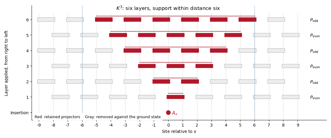
Retained bond projectors in the six-layer cone of a single-site operator under three applications of K
. Details. 
Let and take , so the local projector cone in a frustration-free chain for does not contain . It follows that . The exact bra identity from (ii) and this commutation giveSince , subtracting the product of expectations yieldsThus the exponential clustering from layered projectors bound isThe connected correlation function therefore has correlation length at most in lattice-spacing units. In particular for a small spectral gap. The same-site case is covered by the elementary bound .
Define the orthonormal history basiswhere . Orthogonality follows from the distinct unary quantum clock strings, regardless of overlaps between the computational states.
The initialization term acts diagonally:Each propagation term only couples the two clock strings adjacent to its step. The gate and its adjoint giveand for . The same calculation covers the two endpoint terms.
Thus both Hamiltonians preserve , and in the history basis their restrictions areThis history-subspace propagation Hamiltonian is a path graph Laplacian with a factor . The specified two-clock endpoint formulas assume ; a shorter circuit can first be padded with identity gates.
The matrix is an orthogonal projection. Its eigenvalues areIts unique ground state in is , and its spectral gap is one.
The history-subspace propagation Hamiltonian has diagonal entries at the endpoints and in the interior, and nearest-neighbour entries . The spectrum of a path propagation Hamiltonian isTo see the indexing directly, set and . The interior difference equation gives . The endpoint equations correspond to and , both satisfied by these . The distinct eigenvalues and their nonzero eigenvectors exhaust the matrix.
The supplied path-matrix hint sums through while listing a basis ending at . That last summand would introduce an extra vertex. The matrix derived in (a) has exactly edges and vertices, as used here; this also proves the needed spectrum without relying on the misindexed summation.
Because each term in the history-subspace propagation Hamiltonian is positive semidefinite, the uniform history vector has zero energy and is a ground state:Indeed every edge term annihilates the uniform coefficients. Conversely, a zero-energy vector must have equal coefficients across every edge of the connected path, so this computational history state is the unique ground state in . It coherently records every intermediate state of the quantum circuit.
In the history basis, is a Hermitian tridiagonal matrix. Its first diagonal entry is , its interior entries are , its last entry is , and each off-diagonal entry is .
The Gershgorin disc theorem confines the first row's eigenvalue to , the interior rows to , and the last row to . For , the first disc is disjoint from all the others and therefore contains exactly one eigenvalue. Since is positive semidefinite, that eigenvalue is the ground state energy. All other eigenvalues are at least , while the lowest is at most . Hence the Gershgorin gap bound for an adiabatic history path givesThis argument also covers , where the first disc is the isolated point zero.
Part (a) shows that is invariant throughout the interpolation. As the Hamiltonians are Hermitian, is invariant as well: evolution starting in has no leakage into other sectors. The quantum adiabatic theorem may therefore be applied using the restricted spectral gap, even if other sectors of the full Hamiltonian have different low-energy levels.
Combining (b)(iv) with the supplied bound for gives for a constant . The matrix has diagonal entries and off-diagonal entries . Its Gershgorin discs all lie in , so . Thus the runtime criterion for adiabatic preparation of a computational history state is satisfied bywith a sufficiently large constant.
Starting from the supplied initial ground state , the resulting state obeysHere the trace norm follows the question's convention; the conventional trace distance is half this norm. The Hamiltonian has explicitly specified terms, each acting on at most five qubits, so its description and the runtime are polynomial in circuit size. If is polynomially bounded, the whole preparation has polynomial cost. The initial computational input is assumed to have been prepared, as in the premise of the quantum adiabatic theorem.
A promise problem belongs to QMA if there are polynomials and a uniform family of quantum circuits of size at most , taking a -qubit witness and clean ancillas, with one output qubit interpreted as acceptance, such thatNo condition is imposed outside the promise. The witness may be an arbitrary density operator, and the verifier is efficient but need not know how to prepare an honest witness. Pure witnesses suffice for completeness because the acceptance probability is linear in the witness. QMA is quantum verification with polynomially many witness qubits and a constant completeness-soundness gap.
Interpret the high-success formulation as completeness at least and soundness at most , where for a growing polynomial . This is the standard error-reduction claim. Literally placing around a success probability approaching one supplies no useful lower bound; it is the failure probability that must be inverse-polynomially small.
Let be the quantum verifier acceptance operator acting on one witness register:Acceptance on is . On a NO instance, ; on a YES instance, an honest witness has acceptance at least .
Ask for witness registers, with odd, run independently on each register with fresh ancillas, and accept a strict majority. The QMA parallel repetition with entangled witnesses acceptance operator isDiagonalize . In the tensor-product eigenbasis, an eigenvalue of is the majority probability for independent Bernoulli random variables with parameters equal to the selected eigenvalues of . On a NO instance every parameter is at most . Coupling these variables using independent uniform random numbers shows that their upper majority tail is bounded by the tail with every parameter . This bounds the operator norm and therefore covers every supplied witness, including a witness entangled across the registers. No independence assumption about a dishonest witness is being made.
For a valid Chernoff bound, if is a sum of independent Bernoulli variables of parameter at most , Markov's inequality applied to yieldsAn honest product witness on a YES instance gives independent trials with rejection probability at most , so its failure probability has the same bound. The printed concentration bound is not valid as stated: for five trials at parameter , the upper-majority probability is . The valid bound above suffices for a rigorous proof.
Choose the next odd integer above . ThenThe witness length and circuit size increase by only ; the majority calculation has polynomial overhead. Conversely, inverse-polynomial failure probability is at most for all sufficiently large input lengths. Finitely many smaller lengths can be handled by hard-wired verifiers, giving the usual constants. Hence the two definitions give the same class QMA. The same QMA error reduction argument also yields exponentially small failure with polynomially many copies.
The local Hamiltonian problem is a promise problem specified by a sum on qubits, where is polynomial in , each Hermitian term acts on at most a fixed number of qubits, and the terms and two thresholds are described with polynomially many bits. The promise gap satisfies . In a convenient normalization, . The task is to distinguishThere is no required answer when the minimum energy lies between the thresholds. A formulation with Hermitian terms of polynomially bounded norm is equivalent: shift each term by a known scalar lower bound and rescale all terms by a polynomial bound to obtain positive semidefinite terms of norm at most one, while shifting and rescaling in parallel. The promise gap remains inverse-polynomial.
Use an -qubit state as the witness. Uniformly choose a term and perform the two-outcome positive operator-valued measure . Regard the second outcome as an energy flag. For witness , its probability isThis is an efficient local-energy measurement verification: a unitary operator on the relevant qubits and one ancilla qubit can implement the measurement using the isometryThe local dimension is constant; the term matrices and the measurement can be approximated to inverse-polynomial accuracy. Uniform choice of and the classical threshold comparison also have polynomial overhead.
SetIn the nontrivial case , is inverse-polynomial. Cases outside this energy range are decided directly from .
Ask for witness registers, measure an independently sampled local term on each, and accept if the mean number of energy flags is at most . An honest product ground state on a YES instance has flag probability at most . The Hoeffding inequality gives failure at most . For completeness, the required Bernoulli concentration estimate follows by bounding the centered log moment-generating function : and is a tilted Bernoulli variance, at most . Hence ; exponential Markov's inequality optimized at yields , and the lower-tail version follows in the same way.
Soundness must also cover entangled witness registers. The averaged flag effect is . All its eigenvalues are at least on a NO instance. The repeated verifier's acceptance effect is a polynomial in the commuting tensor-factor operators and . In their product eigenbasis its eigenvalues are lower-tail probabilities of independent Bernoulli variables whose parameters are each at least . Their lower tail is bounded by the identical-parameter tail at , using the same uniform-variable coupling as in QMA parallel repetition with entangled witnesses. Therefore its operator norm is at most , which bounds acceptance for any entangled witness.
Choosinggives completeness at least and soundness at most . A slightly larger constant absorbs implementation errors; for example, approximate each flag effect in norm to at most , retain a gap at least , and increase by a constant factor. The total witness length and circuit size are polynomial. Thus
Here is a finite-dimensional form of the Kitaev geometrical lemma. Let be positive operators, with nullspaces and all positive eigenvalues at least . First assume . Let be the orthogonal projections onto those nullspaces, and define their smallest angle between two subspaces byIf either nullspace is zero, set . Then
To prove it, spectral decomposition gives and . Write and . For every vector ,Thus . Since is positive semidefinite, each of its eigenvalues lies in , so . Consequentlyas claimed.
If there is a common nullspace , restrict to and define the angle between and there. The same proof bounds the smallest positive eigenvalue of by , while is its zero-energy subspace. This version gives a spectral gap above a possibly degenerate ground state space.
Use the Fourier transform convention and define the spectral filtering of Hamiltonian terms byThe normalization means . Since is real and nonnegative, . Thus the stated positive-frequency cutoff also implies for . The integral exists in operator norm, because its integrand has norm at most .
Let , with for . In this eigenbasis,Every matrix element coupling the unique ground state to an excited state vanishes, in either direction. HenceMoreover, linearity and conservation of under its own Heisenberg picture evolution giveEach filtered term is Hermitian, but it need not remain supported on its original set . The tail assumption supplies stronger long-time control than the integrability used here; no additional tail estimate is needed for the requested identities.
For each interaction neighbourhood, setThen the shell term is . Since , its conjugation leaves fixed, so . Since , is precisely the choice of from (b). Therefore the telescoping local-shell decomposition givesNo limiting interchange is needed: the sum has finitely many shells. Each is supported within the union of supports appearing in together with , because its unitary time evolution acts trivially outside that neighbourhood. The individual shell terms need not commute with the full ground state projector; the full filtered sum does.
The filtered decomposition is not necessarily frustration-free. Commuting with makes an eigenvector of each term; it does not make that eigenvector a lowest-energy state of each term. This is the distinction expressed by commuting with a ground projector does not imply frustration freeness.
For an explicit positive, two-local counterexample on three qubits, let and , and use the two distinct interaction sets and :Both are positive semidefinite and commute with their sum. The total energy on a computational basis vector isThus has unique ground state , energy , and spectral gap . Since , spectral filtering of Hamiltonian terms leaves both terms unchanged for every normalized filter:But , whereas . The global ground state therefore does not minimize , proving that the resulting decomposition is not a frustration-free Hamiltonian.
There is a useful positive result if the original decomposition already is a frustration-free Hamiltonian. If and , then . Averaging its unitary conjugates with nonnegative gives , while . Thus filtering preserves existing frustration freeness; it does not create it for an arbitrary gapped Hamiltonian.
Articles by others on the same topic
There are currently no matching articles.