Use the Gaussian units convention implicit in the coefficient. For a uniform dielectric and a counterion-only electrolyte, the Boltzmann distribution and Poisson-Boltzmann equation areThe reference electric potential is , so ; it is not a prescribed nonzero bulk concentration at infinity. A salt reservoir with additional ion species would require their charge densities as well. With , the cylindrical Laplacian is . Since and , the factors of cancel:Here primes mean differentiation with respect to , and the surface condition is in this coordinate.
Multiply by to obtain a first integral:The two specified far-field limits set . For a solution tending upwards to infinity, take the positive square root. Writing gives , hence the cylindrical counterion-only Poisson-Boltzmann profileFor , and . The corresponding number density is
Apply Gauss's law to a coaxial surface per unit cylinder length. Define the positive accumulated cylindrical screening charge byThe signed outward electric field is , so its magnitude is . In the branch here, , the field is inward andIn this display, is a radial derivative. The quantities are electric charges per unit axial length, not total charges of an infinite cylinder.
At the surface, . Define the charge- Bjerrum length and the Manning parameter . Matching the derivative of the solution givesThus the condensed branch exists only for , and its normalization isThe sign condition is essential: simply squaring would produce a spurious subcritical density. Direct integration using yieldsEquivalently, : the remaining far-field line-charge magnitude is . The Manning condensed fraction is .
Below threshold, no positive-density profile can satisfy those same far-field conditions. Indeed , so a negative initial slope cannot increase to zero. The physical interpretation is the infinite-dilution limit of cylindrical counterions: start with a neutral finite cylindrical cell and send its outer radius to infinity. For , counterions escape to arbitrarily large radii, leaving and no finite condensed charge. The bare-cylinder Boltzmann distribution also shows why its radial normalization diverges in this regime. In the local zero-density limit, ; this does not obey the condensed branch's imposed limits. At the branch has zero amplitude and , rather than .
Consequently the intended counterion condensation result, interpreted as a local infinite-dilution density, isEvery finite neutral cell still contains enough counterions to neutralize the cylinder; the missing residual charge in the local limiting profile is carried to infinity. Taking the infinite-cell limit before the charge integral differs from integrating the entire finite cell first. In SI units, the same reference-charge Bjerrum length is ; the electrostatic prefactors must be changed consistently.
For one small transverse displacement, the elastic energy of the elastic filament iswhere is the filament bending modulus. Its first variation isThe clamped boundary conditions remove the left boundary terms. A force-free and torque-free tip permits independent and , so the natural boundary conditions for a free endpoint are : zero bending moment and transverse shear.
There is an important distinction between an energy minimum and a normal mode. The unloaded higher-order Euler-Lagrange equation is , whose only solution with these four boundary conditions is . A general fluctuating shape is a sum of modes, not one of the stated sinusoidal/hyperbolic functions. To obtain the clamped--free bending modes, extremize the bending Rayleigh quotient, or equivalently with a fixed norm. Its Euler-Lagrange equation isThis is the constrained variational characterization of bending modes. Its four characteristic roots are . Clamping gives and , henceThe free-tip conditions reduce toIts determinant is , so nontrivial modes requireNo zero mode exists, since a cubic satisfying the homogeneous clamp/free conditions is zero. The clamped-free bending spectrum starts with ; bisection or Newton iteration gives , so . Choosing and givesThe second boundary condition follows from the root equation, and is arbitrary until a normalization is chosen.
The bending operator with these boundary conditions is positive and self-adjoint. Twice integrating by parts givesSymmetry implies orthogonality when . Expand and use . Thenby the equipartition theorem. The supplied endpoint identity therefore yields the thermal bending fluctuations of a clamped filament:To evaluate the sum, apply a tip force and minimize . The modified free-end conditions are and , and in the interior. Integration gives , so the tip-force compliance of a cantilever is . On the other hand, minimizing the modal energy minus gives and henceComparison evaluates the fourth inverse-power sum of the cantilever spectrum without truncating the modes:The boxed variance is for the specified single transverse direction. An independent equilibrium check follows by differentiating the Gaussian partition function with respect to : at zero load, reproducing the same result from the static compliance. Keeping only the first normal mode gives about , roughly of the exact variance. With two independent equivalent transverse directions, their summed variance is twice the boxed result. The small-slope model requires , or small compared with the usual three-dimensional persistence length .
Write the deterministic drift of the Adler phase equation as . Its minimum is and its maximum is . For , the zero condition has exactly two solutions in the specified interval:The linearization of a dynamical system at an equilibrium point gives , with . Defining gives , so is stable; , so is unstable. For , is positive everywhere and there are no equilibrium points: the phase runs continuously. This is the distinction between phase locking and running phase dynamics.
With mobility scaled to one, the effective force is . Therefore the tilted washboard potential isFor , its alternating local minima and maxima trap noise-free trajectories in wells. Minima coincide with , and maxima with . For , everywhere: there are no wells and the particle slides down the tilt. The potential is defined on the unwrapped phase and obeys ; it is not a single-valued periodic equilibrium potential on the circle.
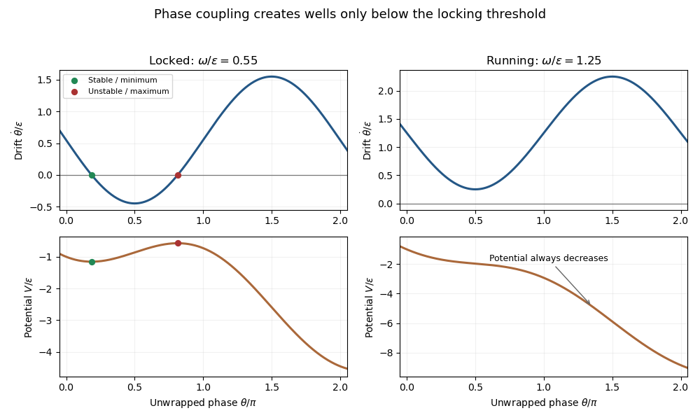
Locked and running Adler phase dynamics, with drift zeros and the corresponding tilted potentials
. Details. 
At the transition , the two equilibrium points merge at in a saddle-node bifurcation. There , so the point is attracting from the left and repelling from the right; a zero linear derivative alone does not establish stable trapping.
For , let and . In a single well, sufficiently small fluctuations obey the linear overdamped Langevin dynamicsThis is an Ornstein-Uhlenbeck process. Its solution isThe mean decays, while the noise integral gives . For , the future-noise contribution is independent of , so . The intrawell phase autocorrelation is thereforeThe connected unnormalized time autocorrelation is just the exponentially decaying second term. The constant first term is necessary because the requested raw correlation is not centered at the equilibrium point. This is the harmonic-well approximation. If a full first-order expansion in is wanted, the quadratic term in the drift is . Local stationarity gives , so the raw correlation gains a constant at that order. The connected correlation is unchanged to first order; the boxed formula is the conventional linearized result rather than a complete nonlinear first-order raw-correlation expansion.
The required time window is long compared with but short compared with the escape time, with the lag also short compared with escape. Fluctuations of size must be small compared with the distance to a neighboring maximum, and the relevant barriers must greatly exceed . For a fixed nonzero noise strength, the unwrapped phase eventually makes phase slips; its raw correlation does not have this stationary infinite-time limit. Thus “large time” here refers to local relaxation within the occupied well, not to the limit after arbitrarily many barrier crossings.
For thermally activated phase slips, the forward saddle is at and the backward saddle at . Their barriers above the same minimum areIn the Kramers escape rate approximation, both saddles have curvature and the minimum has curvature , so the prefactors agree:This is the forward-backward bias of phase slips. It favors forward motion because each forward step lowers the tilted potential by . For , , which gives the same ratio; the exact barrier difference is independent of . These probabilities may be read as rates in a common short observation interval, or as normalized competing exit probabilities. The in the exponent is the noise scale as defined in the Langevin equation; no additional factor is inserted.
Articles by others on the same topic
There are currently no matching articles.