The Taylor series gives . Taking its reciprocal and cancelling the singular term givesThus the apparent singularity at zero is removable, and the first nonzero term is the constant .
The Taylor series of the sine and arctangent give , while . Dividing the two series givesThe first nonzero term after cancellation is the constant .
Factor the numerator as . The Taylor series of the cosine gives . HenceThe first nonzero term is the constant .
True. The symmetric and antisymmetric parts of a matrix are, in Einstein summation convention,They satisfy , and . This works over the real or complex numbers; it uses division by two.
False in general. For symmetric matrices, . The symmetric product criterion for symmetric matrices is therefore . For example,has and despite both factors being symmetric.
True. Set . Exchange , interchange the dummy indices , and use :Thus the matrix congruence preserves symmetry, even when is singular.
True. A symmetric tensor and an antisymmetric tensor are orthogonal under full index contraction. Renaming the two summed indices givesso . This is a scalar statement with both indices summed, not a claim that every individual entrywise product vanishes.
True. Orthogonality gives and , so . Thus is a similar matrix to . If , set . ThenThe transformed eigenvector is nonzero because is invertible. Applying the inverse transformation gives the reverse correspondence, and similar matrices also have the same characteristic polynomial, including algebraic multiplicities of all eigenvalues.
Let mean that the tested person is guilty and mean a positive match. Under the specified model, , and . Bayes' theorem givesThe posterior probability for a unique source after a positive test depends on the number of alternative possible sources as well as the false-positive probability. In particular, the false-positive probability is not the probability of innocence conditional on a positive match.
Under the independent uniform-birthday model, condition on the first person's birthday. Exactly one of the second person's equally likely dates matches, soThis concerns one selected pair; the birthday problem allowing any pair among all guests is a different event.
For matching one specified birthday, each of the other guests avoids the host's date with probability . Independence givesFor this to exceed , the negative logarithm of reverses the inequality on division, giving . Thus the smallest total attendance is , including the host.
The quoted pass probabilities on later attempts are conditional on reaching those attempts. If is the first successful attempt, thenThey sum to , so conditioning on success by the third attempt is essential. The conditional mean of a bounded success time isThe remaining probability represents failing all three attempts and is excluded by this conditioning.
For , integration of the exponential distribution gives its cumulative distribution function:For the event is empty and its probability is zero.
The probability density function is normalized because . Integration by parts gives and . ThereforeThese are the mean and variance of the exponential distribution with rate .
For , use conditional probability and the survival function:It is independent of and equals . This is the memoryless property of the exponential distribution, equivalent here to a constant hazard function .
Assume . The expected net profit per item is . Put and complete the square:This quadratic function has a unique global maximum at . HenceThe calculation uses the expected operating time, rather than replacing lifetime by an arbitrary fixed time.
Let , and . Cross products give plane normals and . Their dot product is and each has norm . Thus the acute angle between two planes isThis is also the interior dihedral angle here: perpendicular to the common edge , the interior wedge lies between the projected directions and . The two outward face normals instead make the supplementary angle.
The face has edge vectors and . Their cross product is , so choose the outward normal vector . The angle between vectors obeysReversing the chosen normal gives the supplementary angle ; the acute angle with the normal line is .
The magnitude of the cross product of two edge vectors is the area of their parallelogram. The triangular face occupies half of it:
With normal vector , the plane through has equation , also satisfied by . Projecting the displacement from the origin onto the unit normal gives the distance from a point to a plane:The perpendicular foot is , which lies in that plane and confirms the distance.
Let be a bounded region with a piecewise smooth closed boundary , and let have continuous first partial derivatives on a neighborhood of its closure. The divergence theorem stateswhere is the outward unit normal vector. The right side is the outward flux; reversing the orientation reverses its sign.
On the radius- sphere, the outward unit normal vector is , so . For a direct surface integral, put , , and . The integral isThe azimuthal integrals are , while and . ThusThe flux of a linear field through a sphere also follows from the equality of the three spherical second moments, without using the divergence theorem.
The divergence is . Since the volume enclosed by a sphere is ,This agrees with the independently computed outward surface integral, as the divergence theorem requires.
The logarithm turns the product defining the factorial into . Since is increasing, each term bounds integrals on its adjacent unit intervals:Summing from to proves the integral bounds for a logarithmic factorial:For , both sides and the empty sum are zero. For , the rectangle diagram gives the same inequalities geometrically. These bounds establish the leading growth, while Stirling's formula gives finer corrections.
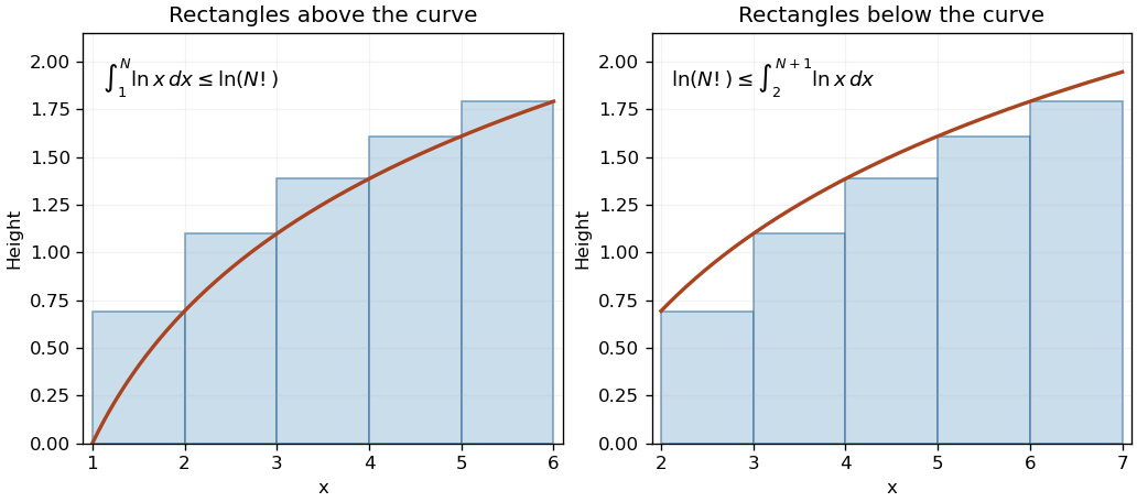

Write . The two data points give the linear equations and . Subtraction and back-substitution giveor , to four significant figures. The six-decimal-place value here is the one printed in the original PDF. Retain guard digits for the estimates below. The fitted coefficients are close to the Stirling's formula values and but need not equal them because the fit absorbs finite- corrections.
Substituting into the fitted factorial logarithm givesThis is an estimate from the requested two-point fit, not an exact factorial evaluation.
For the stated , the leading term dominates the logarithmic correction . ThusThis uses the numerical value specified in the question; such a large logarithm can be computed without constructing the factorial itself.
Separate the even factors from :The double factorial therefore satisfies . Applying the same fit consistently gives
The positive integrand factors into three one-variable functions on a rectangular domain. Fubini's theorem therefore gives
In first-quadrant polar coordinates, , , and the Jacobian determinant contributes . The integrand and area element together become . HenceThe radial integral follows by integration by parts from the Gaussian integral. The isolated undefined ratio at the origin does not affect this convergent double integral.
For fixed , the chain rule and the derivative of the hyperbolic secant giveThus the stated antiderivative holds, with its integration constant independent of but allowed to depend on . At the integrand is zero and the antiderivative is simply constant; the displayed formula with is meant for nonzero .
For and , the preceding antiderivative givesThe integrand is nonnegative, so Tonelli's theorem permits reversing the two integrals without first assuming absolute integrability. Put in the inner integral to obtain the hyperbolic-secant Frullani integral:Here . Near zero, cancellation makes the original integrand ; at infinity it decays exponentially. The finite result therefore also establishes ordinary convergence of the improper integral.
Use separation of variables on intervals avoiding zeros of :Taking the tangent gives the real general solutionEach solution is restricted to an interval where both the original equation and this expression are finite. There is no real constant solution because never vanishes for real .
For , divide by and use the integrating factor , separately on each side of zero. The equation becomes . ThusFor the absolute values may be omitted. The original equation is singular as a first-order evolution equation at zero, so these formulas describe regular intervals with ; extension through zero needs a separate regularity condition.
Rearranging gives . First retain the equilibrium . For every other solution, separation of variables gives , so . HenceA nonconstant solution is defined on any interval where its denominator is nonzero. Dividing by without retaining the equilibrium would lose one solution.
Factor the differential operator as , where . Its homogeneous solutions are , while a nonresonant particular solution is . Imposing the two zero initial conditions gives the exponential forcing response with zero initial dataOne direct derivation avoids a large simultaneous system. Set , so and . The integrating factor gives ; solving with produces the displayed expression. This also verifies the zero derivative at the origin, since .
Now , so the forcing coincides with a homogeneous exponential and requires a resonant exponential particular solution. With as above, and give . ThereforeIntegrating from zero yieldsIts numerator starts at order , ensuring both initial conditions. It is also the finite coalescing-rate limit of the nonresonant exponential forcing response with zero initial data.
Differentiation and factorization give . The exponential and are positive, so the only stationary points are at . The derivative is positive for and negative for , givingThe function is odd, crosses the origin with slope one, and tends to zero from below as and from above as . These facts determine the sketch.
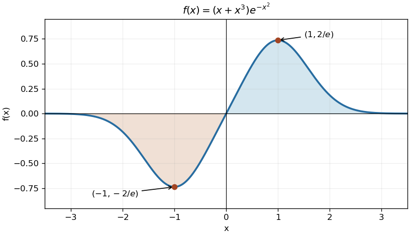
Stationary points and Gaussian decay of the odd polynomial-exponential profile
. Original plot of , with its global extrema marked. Shading indicates the equal and opposite signed areas on the two half-lines. Details.
Since is odd and absolutely integrable, the two signed half-line integrals cancel:Absolute integrability follows from Gaussian decay dominating the polynomial factor; no principal-value interpretation is needed.
Put , so . Then integration by substitution givesThe last two integrals are elementary exponential moments, or values of the Gamma function.
Articles were limited to the first 100 out of 185 total.
Articles by others on the same topic
There are currently no matching articles.