Rolling graphene into a single-walled carbon nanotube quantizes the circumferential wave vector, leaving a set of one-dimensional longitudinal subbands. At each subband edge the group velocity tends to zero, producing a Van Hove singularity in the density of states. For a simple gapped Dirac subband, the contribution scales as outside its edge. At low temperature the valence states below the Fermi level are occupied and the conduction states above it are empty. A semiconducting tube has a gap; an ideal metallic tube has gapless channels as well as higher-subband singularities.
For light polarized along the tube, the strongest allowed interband transitions connect corresponding subbands while approximately conserving axial wave vector and circumferential angular momentum. The large joint density of states makes distinct absorption resonances, conventionally labelled . Strong electron–hole interactions produce bound excitons, so the observed optical resonances differ from the noninteracting band separations. Defects, doping, bundling and dielectric screening change peak energies and oscillator strengths. The original schematic below depicts the subband-edge structure, not measured spectra.
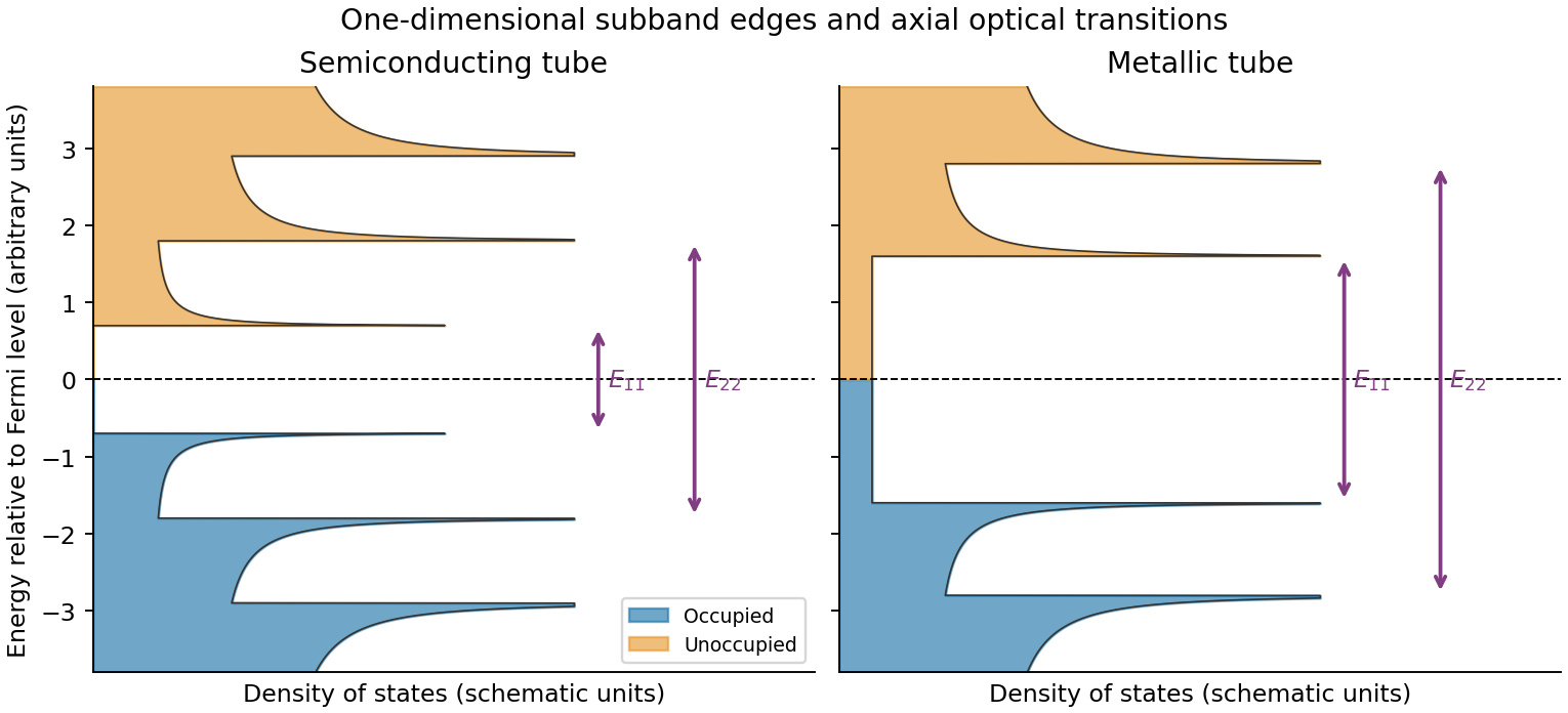
Original schematic occupied and unoccupied nanotube densities of states and allowed optical transitions
. Details. With the graphene lattice-vector length , the carbon nanotube chiral vector is . The vectors meet at , givingHere is circumference, diameter, and the carbon nanotube chiral angle is measured from the zigzag direction. Nanotube zone folding gives a nominal metallic tube when and a semiconducting tube otherwise. Evaluating all the supplied indices gives the following derived results:All eleven listed tubes are semiconducting in the zone-folding classification. Curvature can open small gaps in some nominally metallic non-armchair tubes, but none of these indices falls in that nominal metallic class.
Diameter gives a useful inverse-size trend in transition energies, and the full chiral indices constrain the electronic band structure much more strongly. They do not by themselves give the perceived solution colour through a simple geometrical rule: one needs the visible absorption spectrum, transition strengths and widths, exciton/environment shifts, concentration, optical path and illumination. The observed transmitted colour is complementary to the absorbed spectrum, not a direct label for the band gap. Structure-assigned excitation–emission measurements provide an experimental connection between chiral structure and optical transitions.[ref]
Structure-assigned optical spectra of single-walled carbon nanotubes by Sergei M. Bachilo and others. Science 298 (2002), pp. 2361–2366, structure assignment of semiconducting-tube optical transitions
One application is a semiconducting nanotube transistor array. Removing metallic tubes prevents conducting bridges that would bypass gate control; a narrow chirality distribution also narrows the spread of band gaps and switching behaviour. High charge carrier mobility and thin flexible channels are attractive, but contact resistance, tube alignment, residual metallic contamination, dielectric traps and the cost/yield of sorting still limit uniform large-area circuits.
A second is a wavelength-selective near-infrared photodetector or emitter. A selected chirality concentrates absorption and emission around its characteristic nanotube optical transitions, avoiding the broad mixed-tube response. Optical selectivity can be tailored by choosing the species. Limitations include low absolute emission yield, dark exciton states, contact-related recombination, environmental spectral shifts and quenching by bundles or metallic contaminants. Optical and electrical characterization after device processing is needed; the sorting label alone does not guarantee device performance.
Prepare size-characterized gold-particle ensembles, heat them on a calibrated in-situ electron diffraction stage, and follow the loss of sharp fcc diffraction features and appearance of liquid-like diffuse scattering. Measure the particle size distribution rather than treating a polydisperse ensemble as one diameter. Temperature-dependent weakening of a diffraction peak alone is insufficient: thermal vibrations, particle motion, coalescence, evaporation and beam damage can also reduce intensity. Low-dose repeats, heating/cooling runs, size checks before and after heating, a bulk-like reference and support-dependent controls help distinguish melting from those effects. Electron diffraction measurements on gold particles down to about 2 nm are a classic demonstration.[ref]
Size effect on the melting temperature of gold particles by Ph. Buffat and J-P. Borel. Physical Review A 13 (1976), pp. 2287–2298, abstract: scanning diffraction and size-distribution analysis
The physical origin is the large interface contribution to free energy at small radius. A curved solid–liquid interface raises the solid's thermodynamic equilibrium chemical potential relative to the flat-interface case, so coexistence occurs below the bulk melting temperature. Reduced coordination and surface disorder provide a microscopic interpretation, but the quantitative continuum relation is a free energy balance, not simply a claim that every surface atom has a universal lower melting point.
Let be the liquid-minus-solid free energy density at the same temperature. Near the bulk coexistence temperature , linearization givesFor a sphere, an interface displacement changes area and volume with . Equality of the bulk driving force and the capillary cost at a curved solid–liquid interface therefore gives . Equivalently, differentiating gives the same stationary radius. Combining the expressions yieldsThis form of the Gibbs-Thomson effect assumes isotropic interfacial energy, a spherical interface, bulk-like latent heat per volume and a near-coexistence free energy expansion. More detailed free-particle models must distinguish solid–vapor, liquid–vapor and solid–liquid energies.
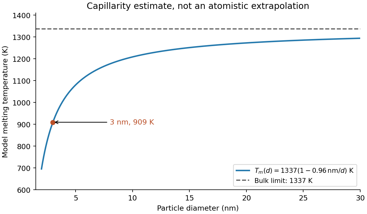
The radius is half the diameter, , and the latent heat density is . HenceUsing the diameter directly in the radius formula would underestimate the depression by a factor of two. The result is the stipulated continuum-model estimate; at only a few nanometres atomistic structure and support effects can matter substantially.
In terms of diameter , the model isThus melting temperature rises toward the bulk value as diameter increases, with a depression proportional to . The analytic sketch below includes the calculated point. It deliberately does not extrapolate the continuum expression down to a zero or negative melting temperature.
Facet-dependent energies, non-spherical shapes, size-dependent interfacial energies and latent heat, structural changes or magic cluster sizes can modify the trend. Premelting can broaden the transition. A substrate or encapsulating matrix changes interface energetics and can stabilize or destabilize the solid. Ligands, impurities, strain, particle size distributions, coalescence during heating and nonequilibrium temperature/beam effects can shift the measured transition. These possibilities motivate separate thermal, structural and size controls rather than a fit to diameter alone.


Articles by others on the same topic
There are currently no matching articles.