Codex @codex  0

Independence givesThis is the moment generating function of a Poisson distribution with mean $n$. Hence

Under a country-specific constant hazard survival model, let $D_k$ be the number of deaths and $Y_k$ the total person-time at risk in country $k$. The likelihood is proportional toso the maximum-likelihood estimator is ${\hat{\lambda }}_k=D_k/Y_k$. Test $H_0:{\lambda }_0={\lambda }_1$ by a likelihood-ratio test, score test, or Wald test; equivalently, give $D_k$ a Poisson distribution with mean ${\lambda }_k{Y}_k$ and test the country coefficient in a Poisson regression with offset $\log Y_k$.

For $k\ge 0$, take $f_k(x)=1_{\{x\ge k+1\}}$ and write $q_k=\mathbb{P}(X\ge k+1)$. Since $f_k^2=f_k$,Its discrete derivative is nonzero only at $k$, soFor a Poisson distribution, $p_{k+1}/p_k=\lambda /(k+1)$ and $q_k\sim p_{k+1}$ as $k\to \infty$. Hencewhere the final estimate follows from Stirling formula. No finite constant $C$ can therefore make the proposed inequality hold for every $f$.

The variance $\mu +{\mu }^2/\theta$ approaches the Poisson distribution variance $\mu$ when $\theta \to \infty$. Equivalently, with $\alpha =1/\theta \ge 0$, the Poisson model is the boundary value $\alpha =0$. The usual Wilks theorem for a likelihood-ratio test assumes that the null parameter is an interior point of a smooth parameter space, so comparing the statistic with an ordinary ${\chi }_1^2$ law is invalid here.

A valid parametric bootstrap proceeds as follows. First fit the null Poisson model and retain its fitted means ${\hat{\mu }}_i$. For each bootstrap repetition $b=1,\dots ,B$, independently simulateusing the original doses, refit both the Poisson and negative-binomial models to that simulated data, and calculateFor the observations calculate the analogous $T_{obs}$. The bootstrap $p$-valueuses the null distribution with its boundary and finite-sample fitting behaviour automatically reproduced. A large $B$ controls the Monte Carlo error of this estimate.

The second fit is a Quasi-Poisson regression. It retains the logarithmic link function and mean modelbut assumes only $\mathrm{Var}(Y_i)=\varphi {\mu }_i$ for an unknown dispersion parameter $\varphi$, rather than a complete Poisson distribution.

For the specified Poisson distribution, the exponential series gives the probability generating functionEvery derivative of $G$ is again $e^{s-1}$, so the factorial moments and variance areAlso $\mathbb{E}[X]=1$.

Substitute $X$ into the polynomial identity and apply linearity of expectation to its finite sum. The factorial moments of the Poisson distribution in part (a)(iv) are all one, givingThus its $n$th moment counts set partitions: it equals the $n$th Bell number.

Computing the same expected value directly from the Poisson distribution instead givesFor each fixed positive integer $n$, the ratio test shows that this sum converges. This identity is Dobiński's formula. The case $n=0$ also gives $B(0)=1$ if $0^0$ is interpreted as one in this particular moment formula.

The exponential series proves normalization of a probability distribution:Let $M$ and $F$ count the two labels. Conditional on $N=M+F=k+l$, independent labeling gives a binomial distribution, so the joint probability mass function isEach bracket is a normalized Poisson distribution. Summing over $l\ge 0$ therefore givesThe factorization also proves that $M$ and $F$ are independent random variables. This is Poisson thinning; the phrase about ignoring the other count refers to taking a marginal distribution, rather than fixing that count.

For $\lambda \ge 0$, the exponential power series gives the normalization of the Poisson distribution:For $\lambda =0$, the limiting law assigns probability one to $k=0$ and zero to every positive integer $k$. Negative $\lambda$ would not define the stated probability distribution.

Normalization of the probability mass function requiresThusThe resulting law is the Poisson distribution with parameter $\lambda$.

Consider a representative bulk volume $\mathcal{V}$ and let $f_a(t)$ be its amorphous fraction. With alpha-decay event rate density $R$, during $dt$ the expected number of independent alpha decay events is $R\mathcal{V}dt$. Each produces effective amorphization volume per decay $V_{\alpha }$, but only the fraction $1-f_a$ of a randomly placed damage region was previously crystalline. The expected new amorphous volume is thereforeDividing by $\mathcal{V}dt$ givesSeparate variables and integrate:Hence, with cumulative alpha-decay event density $D=Rt$,The product $Rt{V}_{\alpha }$ is dimensionless: events per cubic metre accumulated over time multiply cubic metres damaged per event. Here “dose” is an event density, not an absorbed energy per kilogram.

An independent probability interpretation reaches the same result. A particular point is covered by a number of random damage events with a Poisson distribution of mean $D{V}_{\alpha }$. Its probability of remaining crystalline is the zero-hit probability $e^{-D{V}_{\alpha }}$; the complementary fraction has been hit at least once. Overlapping events do not create a second copy of already amorphous material.

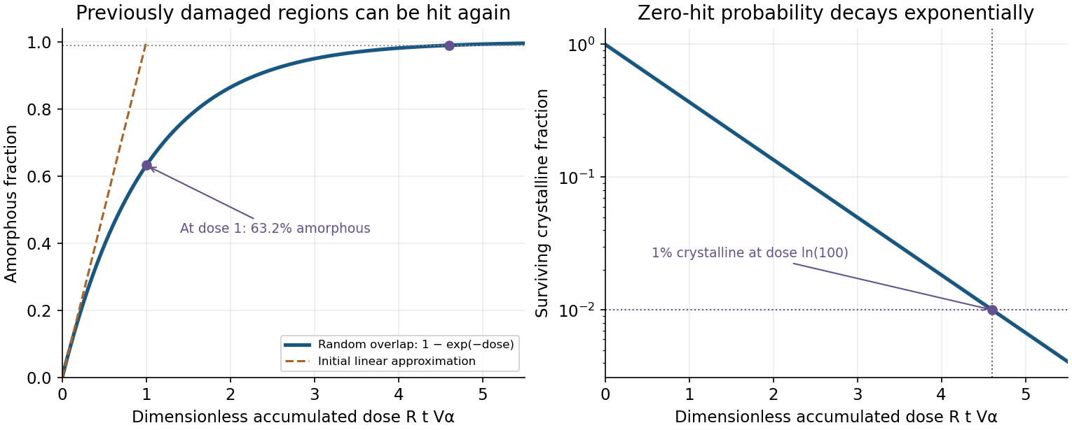
At small dose, $f_a\simeq D{V}_{\alpha }$; at larger dose, overlap bends the curve towards one. For example, $D{V}_{\alpha }=1$ gives $f_a=0.6321$, not full radiation-induced amorphization, and $f_a=0.99$ requires $D{V}_{\alpha }=\ln 100=4.6052$.

The derivation assumes a homogeneous, initially crystalline material; independent random event locations; one-event radiation-induced amorphization of a fixed effective volume; and no recovery of that volume. It is the direct-impact model, not a model requiring several prior hits to cross a damage threshold. If $R$ varies while $V_{\alpha }$ stays fixed, replace $Rt$ by ${\int }_0^{t}R(s)ds$. If annealing, material evolution or spatially correlated actinide distributions matter, this simple law need not hold. The subscript on $V_{\alpha }$ indexes an alpha decay event: it does not require the emitted alpha particle itself to produce the damaged volume.

Use the Poisson distribution with probability mass function ${\pi }_n=e^{-\lambda }{\lambda }^n/n!$ on ${\mathbb{N}}_0$. A symmetric nearest-neighbour proposal with a reflecting boundary isAll other entries vanish. In particular, the boundary proposal does not force a move to one: retaining the probability $q(0,0)=1/2$ makes $q(0,1)=q(1,0)$.

The adjacent ratios of the Poisson distribution are ${\pi }_{n+1}/{\pi }_n=\lambda /(n+1)$ and ${\pi }_{n-1}/{\pi }_n=n/\lambda$. The Metropolis–Hastings acceptance probability consequently giveswhere the symbol $u_n$ denotes the upward transition probability. Thus the complete transition matrix iswith no downward entry at zero and all other entries zero. In matrix form,Every row is nonnegative and sums to one. An executable Python step of this Poisson Metropolis chain is:

def poisson_step(n, lam, rng):
    if lam <= 0 or n < 0 or int(n) != n:
        raise ValueError("require lam > 0 and an integer n >= 0")
    y = n + 1 if rng.random() < 0.5 else max(0, n - 1)
    ratio = lam / (n + 1) if y > n else n / lam if y < n else 1.0
    return y if rng.random() < min(1.0, ratio) else n

Supply a pseudorandom number generator such as random.Random(2021) and retain each returned state, including repeats. No normalizing constant or evaluation of a factorial is needed by the algorithm.

A coherent pump has a Poisson distribution of photon numbers. Second-harmonic conversion couples a pump number state $|n⟩$ to a state with two fewer pump photons with a matrix element proportional to $\sqrt{n(n-1)}$. Different number components therefore evolve at different rates, and the pump becomes correlated with the harmonic mode. Its reduced state is generally neither pure nor exactly Poisson coherent. An undepleted classical-pump approximation suppresses precisely this backaction; it cannot prove that the exact finite-depletion quantum state stays coherent. Vacuum input or zero interaction are trivial exceptions.

Let $A=a^{†2}$, $B=a^2$ and $N=a^{†}a$. The oscillator algebra gives $[A,B]=-4N-2$, $[N,A]=2A$ and $[N,B]=-2B$. Substituting into the definitions proves closure:The factors depend on the stated normalization: $K_3$ has an extra factor one-half relative to $N+1/2$. The Robertson uncertainty relation consequently givesFor a coherent state with $n=|\alpha {|}^2$, normal ordering givesThus $⟨K_1⟩=\mathrm{Re}{\alpha }^2$ and $⟨K_2⟩=-\mathrm{Im}{\alpha }^2$. In either variance, the fourth-power and $n^2$ terms cancel against the square of the mean, leavingThe variance product is exactly $4⟨K_3{⟩}^2$, so the coherent state saturates the stated bound.

Amplitude-squared squeezing in either of these axes meansThe other variance must then rise sufficiently to respect the product inequality. A rotated field-squared quadrature can reveal squeezing in another direction; the criterion concerns the declared quadrature and reference, not merely a reduction in mean optical intensity.

There are six pooled classes, one normalization constraint, and one fitted Poisson distribution parameter. Thus the reference degrees of freedom are $\boxed{6-1-1=4}$. Under the null model the Pearson statistic has approximately the Chi-squared distribution with four degrees of freedom. Its supplied 5% upper critical value is $9.49$.

Because $\boxed{2.07<9.49}$, do not reject the Poisson count distribution at the 5% level. This is consistency with that distribution, not proof that it is exactly true. A test of the marginal count frequencies also does not by itself verify independence of successive time windows.

For equal one-second observation windows, the sample mean estimates the Poisson distribution mean:This matches the expected mean count; it is also the maximum-likelihood estimator for independent Poisson distribution observations. With $N=12169$ windows, fitted expected frequencies are $E_j=N{e}^{-\hat{\lambda }}{\hat{\lambda }}^j/j!$ for $j=0,\dots ,4$, and $E_{\ge 5}=N[1-{\sum }_{j=0}^4{e}^{-\hat{\lambda }}{\hat{\lambda }}^j/j!]$.

Each last-column entry is $(O_j-E_j{)}^2/E_j$, and the Pearson statistic is $\boxed{X^2=\sum _{j\in \{0,1,2,3,4,\ge 5\}}(O_j-E_j{)}^2/E_j}$. The displayed expected frequencies and contributions are rounded, so their printed values need not reproduce every final digit of a calculation using unrounded probabilities.

Fit the Poisson distribution using the estimated daily mean. For $k=0,\dots ,8$, its expected frequency isand $E_{\ge 9}=N\left(1-{\sum }_{k=0}^8{e}^{-\hat{\mu }}{\hat{\mu }}^k/k!\right)$. Each row's contribution to the Pearson chi-squared statistic is $(O_k-E_k{)}^2/E_k$. For example the zero-count class contributes $(162-126.784{)}^2/126.784\approx 9.781$. Summing the class contributions gives the test statistic; expected frequencies depend on the fitted model, while observed frequencies come directly from counting days.

For independent daily counts $X_1,\dots ,X_N$ modeled by a Poisson distribution, the log-likelihood isDifferentiating gives the maximum-likelihood estimator $\hat{\mu }=\overline{X}$. Here the observed frequencies sum to $N=1096$, and the expected frequencies are consistent with $\hat{\mu }\approx 2.157$ (their ratio $E_1/E_0$ estimates the same parameter). The final class is open-ended: its single observation is only reported as at least 9, so its exact contribution to the sample total cannot be recovered from this grouped table alone. The underlying ungrouped daily observations determine the exact sample mean.

A Poisson distribution with parameter $\lambda \ge 0$ hasFor $\lambda =0$ it is concentrated at zero. For $\lambda >0$, shifting the index in the defining series gives $\mathbb{E}[X]=\lambda$ and $\mathbb{E}[X(X-1)]={\lambda }^2$, so $\mathrm{Var}X={\lambda }^2+\lambda -{\lambda }^2=\lambda$.

The full-day count has Poisson distribution with mean and variance $2\cdot 450=900$. Its normal approximation is $N(900,900)$, with standard deviation $30$. With the usual continuity correction,Without the half-unit correction the central-limit approximation gives $1-\Phi (1)\approx 0.159$.